solutions as trigonometric and hyperbolic functions

SearchAdvancedHelp

(0.007 seconds)

11—20 of 25 matching pages

11: 14.20 Conical (or Mehler) Functions

… ►Solutions are known as conical or Mehler functions. … … ►It is an important companion solution to ${𝖯}_{-\frac{1}{2}+\mathrm{i}\tau }^{-\mu }\left(x\right)$ when $\tau$ is large; compare §§14.20(vii), 14.20(viii), and 10.25(iii). … ►

§14.20(v) Trigonometric Expansion

… ►where the inverse trigonometric functions take their principal values. …

12: 10.45 Functions of Imaginary Order

§10.45 Functions of Imaginary Order

… ►and ${\tilde{I}}_{\nu }\left(x\right)$, ${\tilde{K}}_{\nu }\left(x\right)$ are real and linearly independent solutions of (10.45.1): … ►In consequence of (10.45.5)–(10.45.7), ${\tilde{I}}_{\nu }\left(x\right)$ and ${\tilde{K}}_{\nu }\left(x\right)$ comprise a numerically satisfactory pair of solutions of (10.45.1) when $x$ is large, and either ${\tilde{I}}_{\nu }\left(x\right)$ and $(1/\pi )\sinh \left(\pi \nu \right){\tilde{K}}_{\nu }\left(x\right)$, or ${\tilde{I}}_{\nu }\left(x\right)$ and ${\tilde{K}}_{\nu }\left(x\right)$, comprise a numerically satisfactory pair when $x$ is small, depending whether $\nu \ne 0$ or $\nu =0$. … ►In this reference ${\tilde{I}}_{\nu }\left(x\right)$ is denoted by $(1/\pi )\sinh \left(\pi \nu \right)L_{\mathrm{i}\nu }(x)$. …

13: 36.11 Leading-Order Asymptotics

§36.11 Leading-Order Asymptotics

… ►

36.11.2 $${\mathrm{\Psi }}_K\left(𝐱\right)=\sqrt{2\pi }\sum _{j=1}^{j_{\max }(𝐱)}\exp \left(\mathrm{i}\left({\mathrm{\Phi }}_K(t_j(𝐱);𝐱)+\frac{1}{4}\pi {(-1)}^{j+K+1}\right)\right){\left|\frac{{\partial }^2{\mathrm{\Phi }}_K(t_j(𝐱);𝐱)}{{\partial t}^2}\right|}^{-1/2}(1+o\left(1\right)).$$

ⓘ

Symbols:

${\mathrm{\Psi }}_K\left(𝐱\right)$: canonical integral function, $\pi$: the ratio of the circumference of a circle to its diameter, ${\mathrm{\Phi }}_K(t;𝐱)$: cuspoid catastrophe of codimension $K$ , $\exp z$: exponential function, $\mathrm{i}$: imaginary unit, $o\left(x\right)$: order less than, $\frac{\partial f}{\partial x}$: partial derivative of $f$ with respect to $x$ , $\partial x$: partial differential of $x$ , $t$: variable, $K$: codimension and $t_j(𝐱)$: solutions

Permalink:

http://dlmf.nist.gov/36.11.E2

Encodings:

pMML, png, TeX

See also:

Annotations for §36.11 and Ch.36

… ►

36.11.4

ⓘ

Symbols:

${\mathrm{\Psi }}_K\left(𝐱\right)$: canonical integral function, $\pi$: the ratio of the circumference of a circle to its diameter, $\cos z$: cosine function, $\exp z$: exponential function, $o\left(x\right)$: order less than and $x$: real parameter

Referenced by:

§36.11

Permalink:

http://dlmf.nist.gov/36.11.E4

Encodings:

pMML, png, TeX

See also:

Annotations for §36.11, §36.11 and Ch.36

… ►

36.11.6

ⓘ

Symbols:

$\mathrm{\Gamma }\left(z\right)$: gamma function, ${\mathrm{\Psi }}_K\left(𝐱\right)$: canonical integral function, $\pi$: the ratio of the circumference of a circle to its diameter, $\cos z$: cosine function, $o\left(x\right)$: order less than and $z$: real parameter

Permalink:

http://dlmf.nist.gov/36.11.E6

Encodings:

pMML, png, TeX

See also:

Annotations for §36.11, §36.11 and Ch.36

… ►

36.11.8 $${\mathrm{\Psi }}^{(\mathrm{H})}\left(0,0,z\right)=\frac{2\pi }{z}\left(1-\frac{\mathrm{i}}{\sqrt{3}}\exp \left(\frac{1}{27}\mathrm{i}{z}^3\right)+o\left(1\right)\right),$$ $z\to \pm \mathrm{\infty }$.

ⓘ

Symbols:

$\pi$: the ratio of the circumference of a circle to its diameter, $\exp z$: exponential function, ${\mathrm{\Psi }}^{(\mathrm{H})}\left(𝐱\right)$: hyperbolic umbilic canonical integral function, $\mathrm{i}$: imaginary unit, $o\left(x\right)$: order less than and $z$: real parameter

Permalink:

http://dlmf.nist.gov/36.11.E8

Encodings:

pMML, png, TeX

See also:

Annotations for §36.11, §36.11 and Ch.36

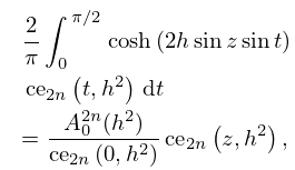
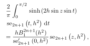
14: 28.10 Integral Equations

… ►

§28.10(i) Equations with Elementary Kernels

… ►

28.10.2 $$\frac{2}{\pi }{\int }_0^{\pi /2}\cosh \left(2h\sin z\sin t\right){\mathrm{ce}}_{2n}(t,h^2)dt=\frac{A_0^{2n}(h^2)}{{\mathrm{ce}}_{2n}(0,h^2)}{\mathrm{ce}}_{2n}(z,h^2),$$

ⓘ

Symbols:

${\mathrm{ce}}_n(z,q)$: Mathieu function, $\pi$: the ratio of the circumference of a circle to its diameter, $dx$: differential of $x$ , $\cosh z$: hyperbolic cosine function, $\int$: integral, $\sin z$: sine function, $h$: parameter, $n$: integer, $z$: complex variable and $A_m(q)$: Fourier coefficient

A&S Ref:

20.7.21 (in different form)

Permalink:

http://dlmf.nist.gov/28.10.E2

Encodings:

pMML, png, TeX

See also:

Annotations for §28.10(i), §28.10 and Ch.28

… ►

28.10.5 $$\frac{2}{\pi }{\int }_0^{\pi /2}\sinh \left(2h\sin z\sin t\right){\mathrm{se}}_{2n+1}(t,h^2)dt=\frac{h{B}_1^{2n+1}(h^2)}{{\mathrm{se}}_{2n+1}^{\prime }(0,h^2)}{\mathrm{se}}_{2n+1}(z,h^2),$$

ⓘ

Symbols:

${\mathrm{se}}_n(z,q)$: Mathieu function, $\pi$: the ratio of the circumference of a circle to its diameter, $dx$: differential of $x$ , $\sinh z$: hyperbolic sine function, $\int$: integral, $\sin z$: sine function, $h$: parameter, $n$: integer, $z$: complex variable and $B_m(q)$: Fourier coefficient

A&S Ref:

20.7.23 (in different form)

Permalink:

http://dlmf.nist.gov/28.10.E5

Encodings:

pMML, png, TeX

See also:

Annotations for §28.10(i), §28.10 and Ch.28

… ►

§28.10(ii) Equations with Bessel-Function Kernels

… ►

§28.10(iii) Further Equations

…

15: 10.20 Uniform Asymptotic Expansions for Large Order

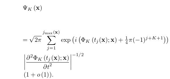
§10.20 Uniform Asymptotic Expansions for Large Order

… ►Define $\zeta =\zeta (z)$ to be the solution of the differential equation … ►In this way there is less usage of many-valued functions. … ►where ${\tau }_0=1.19968\mathrm{\dots }$ is the positive root of the equation $\tau =\coth \tau$. … ►

§10.20(iii) Double Asymptotic Properties

…

16: 32.2 Differential Equations

… ►An equation is said to have the Painlevé property if all its solutions are free from movable branch points; the solutions may have movable poles or movable isolated essential singularities (§1.10(iii)), however. … ►For arbitrary values of the parameters $\alpha$, $\beta$, $\gamma$, and $\delta$, the general solutions of ${\text{P}}_{\text{I}}$–${\text{P}}_{\text{VI}}$ are transcendental, that is, they cannot be expressed in closed-form elementary functions. However, for special values of the parameters, equations ${\text{P}}_{\text{II}}$–${\text{P}}_{\text{VI}}$ have special solutions in terms of elementary functions, or special functions defined elsewhere in the DLMF. … ►In ${\text{P}}_{\text{V}}$, if $w(z)={(\coth u(\zeta ))}^2$ with $\zeta =\ln z$, then … ►Let …

17: Bibliography L

… ►

The solutions of the Mathieu equation with a complex variable and at least one parameter large. Trans. Amer. Math. Soc. 36 (3), pp. 637–695.

ⓘ

External Links:

ISSN 0002-9947, FullText, MathReview Entry, ZentralBlatt

Referenced by:

§28.8(iv).

Encodings:

BibTeX

… ►

Exact operator solution of the Calogero-Sutherland model. Comm. Math. Phys. 178 (2), pp. 425–452.

ⓘ

Notes:

For a Maple implementation of the algorithm given in this paper for Jack and zonal polynomials see Zeilberger (website).

External Links:

ISSN 0010-3616, Link, MathReview (Kazuhiro Hikami), ZentralBlatt

Referenced by:

§35.12.

Encodings:

BibTeX

… ►

Well-posedness and blow-up solutions for an integrable nonlinearly dispersive model wave equation. J. Differential Equations 162 (1), pp. 27–63.

ⓘ

External Links:

ISSN 0022-0396, Document, MathReview (John Albert), ZentralBlatt

Referenced by:

§22.19(iii).

Encodings:

BibTeX

… ►

A note on the computation of integrals involving products of trigonometric and Bessel functions. Math. Comp. 27 (124), pp. 871–872.

ⓘ

External Links:

ISSN 0025-5718, FullText, Document, MathReview, ZentralBlatt

Referenced by:

§10.74(vii).

Encodings:

BibTeX

… ►

Uniform approximations of Bernoulli and Euler polynomials in terms of hyperbolic functions. Stud. Appl. Math. 103 (3), pp. 241–258.

ⓘ

External Links:

ISSN 0022-2526, Document, Link, MathReview, ZentralBlatt

Referenced by:

§24.11, §24.11.

Encodings:

BibTeX

…

18: 22.19 Physical Applications

… ►The bounded $(-\pi \le \theta \le \pi )$ oscillatory solution of (22.19.1) is traditionally written … ►This formulation gives the bounded and unbounded solutions from the same formula (22.19.3), for $k\ge 1$ and $k\le 1$, respectively. … ►Both the $\mathrm{dn}$ and $\mathrm{cn}$ solutions approach $a\mathrm{sech}t$ as $a\to \sqrt{2/\beta }$ from the appropriate directions. … ►Many nonlinear ordinary and partial differential equations have solutions that may be expressed in terms of Jacobian elliptic functions. … ►Hyperelliptic functions $u(z)$ are solutions of the equation $z={\int }_0^u{(f(x))}^{-1/2}dx$, where $f(x)$ is a polynomial of degree higher than 4. …

19: 14.3 Definitions and Hypergeometric Representations

… ►The following are real-valued solutions of (14.2.2) when $\mu$, $\nu \in ℝ$ and . … ►The following are solutions of (14.2.2) when $\mu$, $\nu \in ℝ$ and . … ►As standard solutions of (14.2.2) we take the pair and , where … ►

§14.3(iii) Alternative Hypergeometric Representations

… ►

§14.3(iv) Relations to Other Functions

…

20: Errata

… ►

In the first sentence of this subsection, the constraint $\sinh \left|\beta \right|\le \mathrm{\ell }$ has been replaced with $\left|\mathrm{\Re }\beta \right|+\left|\mathrm{\Im }\beta \right|\le \mathrm{\ell }$.

… ►

10.22.72 $${\int }_0^{\mathrm{\infty }}{J}_{\mu }\left(at\right)J_{\nu }\left(bt\right)J_{\nu }\left(ct\right)t^{1-\mu }dt=\frac{{(bc)}^{\mu -1}\sin \left((\mu -\nu )\pi \right){(\sinh \chi )}^{\mu -\frac{1}{2}}}{{(\frac{1}{2}{\pi }^3)}^{\frac{1}{2}}{a}^{\mu }}{\mathrm{e}}^{(\mu -\frac{1}{2})\mathrm{i}\pi }{Q}_{\nu -\frac{1}{2}}^{\frac{1}{2}-\mu }\left(\cosh \chi \right),$$ $\mathrm{\Re }\mu >-\frac{1}{2},\mathrm{\Re }\nu >-1,a>b+c,\cosh \chi =(a^2-b^2-c^2)/(2bc)$

Originally, the factor on the right-hand side was written as $\frac{{(bc)}^{\mu -1}\cos \left(\nu \pi \right){(\sinh \chi )}^{\mu -\frac{1}{2}}}{{(\frac{1}{2}{\pi }^3)}^{\frac{1}{2}}{a}^{\mu }}$, which was taken directly from Watson (1944, p. 412, (13.46.5)), who uses a different normalization for the associated Legendre function of the second kind $Q_{\nu }^{\mu }$. Watson’s $Q_{\nu }^{\mu }$ equals $\frac{\sin \left((\nu +\mu )\pi \right)}{\sin \left(\nu \pi \right)}{\mathrm{e}}^{-\mu \pi \mathrm{i}}{Q}_{\nu }^{\mu }$ in the DLMF.

Reported by Arun Ravishankar on 2018-10-22

… ►

Scales were corrected in all figures. The interval $-8.4\le \frac{x-y}{\sqrt{2}}\le 8.4$ was replaced by $-12.0\le \frac{x-y}{\sqrt{2}}\le 12.0$ and $-12.7\le \frac{x+y}{\sqrt{2}}\le 4.2$ replaced by $-18.0\le \frac{x+y}{\sqrt{2}}\le 6.0$. All plots and interactive visualizations were regenerated to improve image quality.

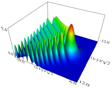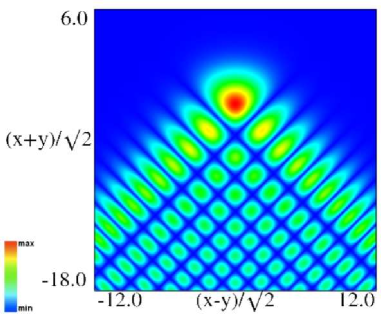
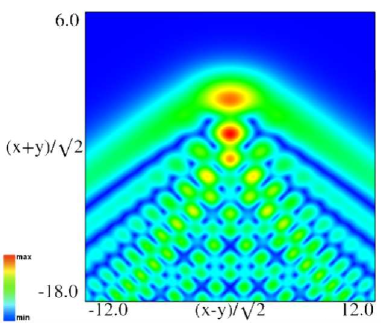
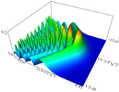
(a) Density plot.	(b) 3D plot.

Figure 36.3.9: Modulus of hyperbolic umbilic canonical integral function $|{\mathrm{\Psi }}^{(\mathrm{H})}\left(x,y,0\right)|$.

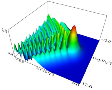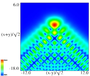
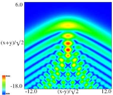
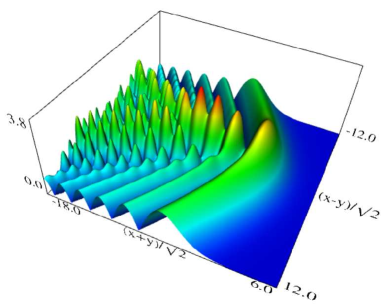
(a) Density plot.	(b) 3D plot.

Figure 36.3.10: Modulus of hyperbolic umbilic canonical integral function $|{\mathrm{\Psi }}^{(\mathrm{H})}\left(x,y,1\right)|$.

(a) Density plot.	(b) 3D plot.

Figure 36.3.11: Modulus of hyperbolic umbilic canonical integral function $|{\mathrm{\Psi }}^{(\mathrm{H})}\left(x,y,2\right)|$.

(a) Density plot.	(b) 3D plot.

Figure 36.3.12: Modulus of hyperbolic umbilic canonical integral function $|{\mathrm{\Psi }}^{(\mathrm{H})}\left(x,y,3\right)|$.

Reported 2016-09-12 by Dan Piponi.

… ►

The first paragraph has been rewritten to correct reported errors. The new version is reproduced here.

Let $p$ $(\ne 0)$ and $q$ be real constants and

4.43.1

$A={\left(-\frac{4}{3}p\right)}^{1/2},$

$B={\left(\frac{4}{3}p\right)}^{1/2}.$

The roots of

4.43.2 $$z^3+pz+q=0$$

are:

1. $A\sin a$, $A\sin \left(a+\frac{2}{3}\pi \right)$, and $A\sin \left(a+\frac{4}{3}\pi \right)$, with $\sin \left(3a\right)=4q/A^3$, when $4p^3+27q^2\le 0$.

2. $A\cosh a$, $A\cosh \left(a+\frac{2}{3}\pi \mathrm{i}\right)$, and $A\cosh \left(a+\frac{4}{3}\pi \mathrm{i}\right)$, with $\cosh \left(3a\right)=-4q/A^3$, when , , and $4p^3+27q^2>0$.

3. $B\sinh a$, $B\sinh \left(a+\frac{2}{3}\pi \mathrm{i}\right)$, and $B\sinh \left(a+\frac{4}{3}\pi \mathrm{i}\right)$, with $\sinh \left(3a\right)=-4q/B^3$, when $p>0$.

Note that in Case (a) all the roots are real, whereas in Cases (b) and (c) there is one real root and a conjugate pair of complex roots. See also §1.11(iii).

Reported 2014-10-31 by Masataka Urago.

… ►

Originally the limiting form for $\mathrm{sc}(z,k)$ in the last line of this table was incorrect ($\cosh z$, instead of $\sinh z$).

$\mathrm{sn}(z,k)$ $\to$	$\tanh z$	$\mathrm{cd}(z,k)$ $\to$	$1$	$\mathrm{dc}(z,k)$ $\to$	$1$	$\mathrm{ns}(z,k)$ $\to$	$\coth z$
$\mathrm{cn}(z,k)$ $\to$	$\mathrm{sech}z$	$\mathrm{sd}(z,k)$ $\to$	$\sinh z$	$\mathrm{nc}(z,k)$ $\to$	$\cosh z$	$\mathrm{ds}(z,k)$ $\to$	$\mathrm{csch}z$
$\mathrm{dn}(z,k)$ $\to$	$\mathrm{sech}z$	$\mathrm{nd}(z,k)$ $\to$	$\cosh z$	$\mathrm{sc}(z,k)$ $\to$	$\sinh z$	$\mathrm{cs}(z,k)$ $\to$	$\mathrm{csch}z$

Reported 2010-11-23.

…