scaled
(0.001 seconds)
31—40 of 61 matching pages
31: 5.23 Approximations
…
►See Schmelzer and Trefethen (2007) for a survey of rational approximations to various scaled versions of .
…
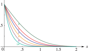
32: 7.18 Repeated Integrals of the Complementary Error Function
33: 10.16 Relations to Other Functions
34: Philip J. Davis
…
►The surface color map can be changed from height-based to phase-based for complex valued functions, and density plots can be generated through strategic scaling.
…
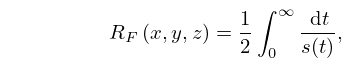
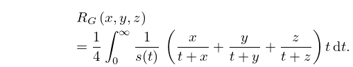
35: 19.16 Definitions
36: 21.9 Integrable Equations
…
►All quantities are made dimensionless by a suitable scaling transformation.
…
37: Mathematical Introduction
…
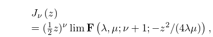
►For example, for the hypergeometric function we often use the notation (§15.2(i)) in place of the more conventional or .
This is because is akin to the notation used for Bessel functions (§10.2(ii)), inasmuch as is an entire function of each of its parameters , , and : this results in fewer restrictions and simpler equations.
…
38: 3.10 Continued Fractions
…
►However, this may be unstable; also overflow and underflow may occur when evaluating and (making it necessary to re-scale from time to time).
…
►In contrast to the preceding algorithms in this subsection no scaling problems arise and no a priori information is needed.
…
►Again, no scaling problems arise and no a priori information is needed.
…
39: 10.22 Integrals
…
►
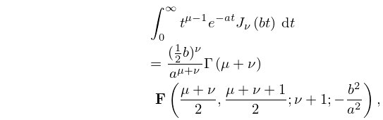
10.22.49
,
►
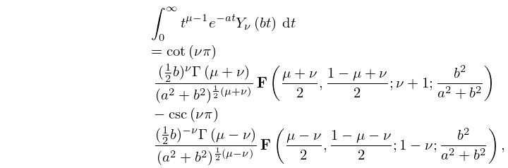
10.22.50
.
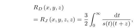
►For the hypergeometric function see §15.2(i).
…
►
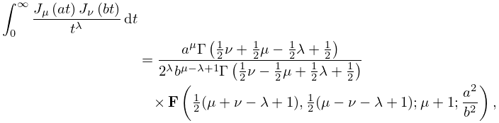
10.22.56
, .
…
►
10.22.64
…
40: 16.2 Definition and Analytic Properties
…
►
16.2.5
…
