on the left (or right)
(0.001 seconds)
11—20 of 78 matching pages
11: 2.4 Contour Integrals
…
►The most successful results are obtained on moving the integration contour as far to the left as possible.
…
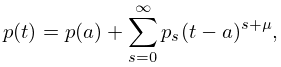
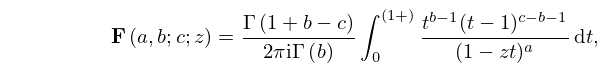
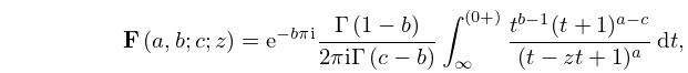
►Let denote the path for the contour integral
►
(a)
…
►
2.4.10
…
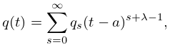
►
In a neighborhood of
2.4.11
with , , , and the branches of and continuous and constructed with as along .
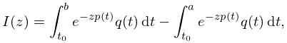
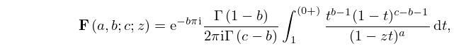
2.4.14
…
12: 15.6 Integral Representations
13: 16.5 Integral Representations and Integrals
…
►Then the integral converges when provided that , or when provided that , and provides an integral representation of the left-hand side with these conditions.
…
►In the case the left-hand side of (16.5.1) is an entire function, and the right-hand side supplies an integral representation valid when .
In the case the right-hand side of (16.5.1) supplies the analytic continuation of the left-hand side from the open unit disk to the sector ; compare §16.2(iii).
Lastly, when the right-hand side of (16.5.1) can be regarded as the definition of the (customarily undefined) left-hand side.
In this event, the formal power-series expansion of the left-hand side (obtained from (16.2.1)) is the asymptotic expansion of the right-hand side as in the sector , where is an arbitrary small positive constant.
…
14: 5.19 Mathematical Applications
15: 10.59 Integrals
…
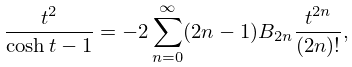
16: 24.19 Methods of Computation
…
►
•
…
17: 3.2 Linear Algebra
…
►A nonzero vector is called a left eigenvector of corresponding to the eigenvalue if or, equivalently, .
…
…
►where and are the normalized right and left eigenvectors of corresponding to the eigenvalue .
…When is a symmetric matrix, the left and right eigenvectors coincide, yielding , and the calculation of its eigenvalues is a well-conditioned problem.
…
18: 1.8 Fourier Series
…
►at every point at which has both a left-hand derivative (that is, (1.4.4) applies when ) and a right-hand derivative (that is, (1.4.4) applies when ).
…
…
19: 4.10 Integrals
20: 8.7 Series Expansions
…
►
8.7.6
, .
…
