…
►
28.22.9
►
28.22.10
…
►
►
…
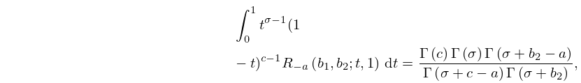
►Here
is given by (
28.14.1) with
, and
is given by (
28.24.1) with
,
, and
chosen so that
, where the
maximum is taken over all integers
.
…
…
►
3.3.12
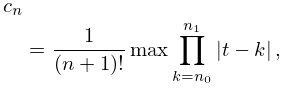
►where the
maximum is taken over
-intervals given in the formulas below.
…
►
…
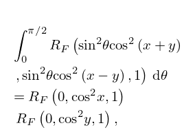
►For example, for
coincident points the limiting form is given by
.
…
►
3.3.44
…
…
►where
.
…To generate
the quantities
are needed.
…
►Complex orthogonal polynomials
of degree
, in
that satisfy the orthogonality condition
…
►A frequent problem with contour integrals is heavy cancellation, which occurs especially when the value of the integral is exponentially small compared with the
maximum absolute value of the integrand.
To avoid cancellation we try to deform the path to pass through a saddle point in such a way that the
maximum contribution of the integrand is derived from the neighborhood of the saddle point.
…
…
►A sufficient condition for
to be the minimax polynomial is that
attains its
maximum at
distinct points in
and
changes sign at these consecutive maxima.
…
►(Thus the
are approximations to
, where
is the
maximum value of
on
.)
…
►More precisely, it is known that for the interval
, the ratio of the
maximum value of the remainder
…to the
maximum error of the minimax polynomial
is bounded by
, where
is the
th
Lebesgue constant for Fourier series; see §
1.8(i).
…
►and
is the
maximum of
on
.
…
