locally%20integrable

SearchAdvancedHelp

(0.001 seconds)

21—30 of 358 matching pages

21: 13.29 Methods of Computation

… ►A comprehensive and powerful approach is to integrate the differential equations (13.2.1) and (13.14.1) by direct numerical methods. As described in §3.7(ii), to insure stability the integration path must be chosen in such a way that as we proceed along it the wanted solution grows in magnitude at least as fast as all other solutions of the differential equation. ►For $M(a,b,z)$ and $M_{\kappa ,\mu }\left(z\right)$ this means that in the sector $|\mathrm{ph}z|\le \pi$ we may integrate along outward rays from the origin with initial values obtained from (13.2.2) and (13.14.2). … ►In the sector the integration has to be towards the origin, with starting values computed from asymptotic expansions (§§13.7 and 13.19). On the rays $\mathrm{ph}z=\pm \frac{1}{2}\pi$, integration can proceed in either direction. …

22: 28.8 Asymptotic Expansions for Large $q$

… ►

28.8.6 $${\widehat{C}}_m\sim {\left(\frac{\pi h}{2{(m!)}^2}\right)}^{1/4}{\left(1+\frac{2m+1}{8h}+\frac{m^4+2m^3+263m^2+262m+108}{2048h^2}+\mathrm{\cdots }\right)}^{-1/2},$$

ⓘ

Defines:

${\widehat{C}}_m$: coefficient (locally)

Symbols:

$\sim$: Poincaré asymptotic expansion, $\pi$: the ratio of the circumference of a circle to its diameter, $!$: factorial (as in $n!$), $m$: integer and $h$: parameter

A&S Ref:

20.9.19 (in slightly different form)

Permalink:

http://dlmf.nist.gov/28.8.E6

Encodings:

pMML, png, TeX

See also:

Annotations for §28.8(ii), §28.8 and Ch.28

►

28.8.7 $${\widehat{S}}_m\sim {\left(\frac{\pi h}{2{(m!)}^2}\right)}^{1/4}{\left(1-\frac{2m+1}{8h}+\frac{m^4+2m^3-121m^2-122m-84}{2048h^2}+\mathrm{\cdots }\right)}^{-1/2}.$$

ⓘ

Defines:

${\widehat{S}}_m$: coefficient (locally)

Symbols:

$\sim$: Poincaré asymptotic expansion, $\pi$: the ratio of the circumference of a circle to its diameter, $!$: factorial (as in $n!$), $m$: integer and $h$: parameter

A&S Ref:

20.9.20 (in slightly different form)

Referenced by:

§28.8(ii), Erratum (V1.1.10) for Sections 28.6(i), 28.6(ii), 28.8(i), 28.8(ii)

Permalink:

http://dlmf.nist.gov/28.8.E7

Encodings:

pMML, png, TeX

See also:

Annotations for §28.8(ii), §28.8 and Ch.28

… ►

28.8.9 $$W_m^{\pm }(x)=\frac{{\mathrm{e}}^{\pm 2h\sin x}}{{(\cos x)}^{m+1}}\{\begin{array}{cc}{\left(\cos \left(\frac{1}{2}x+\frac{1}{4}\pi \right)\right)}^{2m+1},\hfill & \\ {\left(\sin \left(\frac{1}{2}x+\frac{1}{4}\pi \right)\right)}^{2m+1},\hfill & \end{array}$$

ⓘ

Defines:

$W_m^{\pm }$: function (locally)

Symbols:

$\pi$: the ratio of the circumference of a circle to its diameter, $\cos z$: cosine function, $\mathrm{e}$: base of natural logarithm, $\sin z$: sine function, $m$: integer, $h$: parameter and $x$: real variable

A&S Ref:

20.9.13 (in slightly different form)

Permalink:

http://dlmf.nist.gov/28.8.E9

Encodings:

pMML, png, TeX

See also:

Annotations for §28.8(iii), §28.8 and Ch.28

… ►

28.8.11 $$P_m(x)\sim 1+\frac{s}{2^{3}h{\cos }^{2}x}+\frac{1}{h^2}\left(\frac{s^4+86s^2+105}{2^{11}{\cos }^{4}x}-\frac{s^4+22s^2+57}{2^{11}{\cos }^{2}x}\right)+\mathrm{\cdots },$$

ⓘ

Defines:

$P_m(x)$ (locally)

Symbols:

$\sim$: Poincaré asymptotic expansion, $\cos z$: cosine function, $m$: integer, $h$: parameter and $x$: real variable

A&S Ref:

20.9.14 (in different form)

Permalink:

http://dlmf.nist.gov/28.8.E11

Encodings:

pMML, png, TeX

See also:

Annotations for §28.8(iii), §28.8 and Ch.28

►

28.8.12 $$Q_m(x)\sim \frac{\sin x}{{\cos }^{2}x}\left(\frac{1}{2^{5}h}(s^2+3)+\frac{1}{2^9{h}^2}\left(s^3+3s+\frac{4s^3+44s}{{\cos }^{2}x}\right)\right)+\mathrm{\cdots }.$$

ⓘ

Defines:

$Q_m(x)$ (locally)

Symbols:

$\sim$: Poincaré asymptotic expansion, $\cos z$: cosine function, $\sin z$: sine function, $m$: integer, $h$: parameter and $x$: real variable

A&S Ref:

20.9.14 (in different form)

Permalink:

http://dlmf.nist.gov/28.8.E12

Encodings:

pMML, png, TeX

See also:

Annotations for §28.8(iii), §28.8 and Ch.28

…

23: 2.3 Integrals of a Real Variable

… ►

§2.3(i) Integration by Parts

… ►Then the series obtained by substituting (2.3.7) into (2.3.1) and integrating formally term by term yields an asymptotic expansion: … ►derives from the neighborhood of the minimum of $p(t)$ in the integration range. … ►A uniform approximation can be constructed by quadratic change of integration variable: … ►We replace the limit $\kappa$ by $\mathrm{\infty }$ and integrate term-by-term: …

24: 12.10 Uniform Asymptotic Expansions for Large Parameter

… ►

12.10.8 $${𝒜}_s(t)=\frac{u_s(t)}{{(t^2-1)}^{\frac{3}{2}s}},{ℬ}_s(t)=\frac{v_s(t)}{{(t^2-1)}^{\frac{3}{2}s}},$$

ⓘ

Defines:

${𝒜}_s(t)$: coefficients (locally) and ${ℬ}_s(t)$: coefficients (locally)

Symbols:

$s$: nonnegative integer, $u_s(t)$: solution and $v_s(t)$: solution

Referenced by:

§12.10(iv)

Permalink:

http://dlmf.nist.gov/12.10.E8

Encodings:

pMML, png, TeX

See also:

Annotations for §12.10(ii), §12.10 and Ch.12

… ►

12.10.23 $$\eta =\frac{1}{2}\arccos t-\frac{1}{2}t\sqrt{1-t^2},$$

ⓘ

Defines:

$\eta$ (locally)

Symbols:

$\arccos z$: arccosine function

Referenced by:

§12.10(vii), §12.14(ix)

Permalink:

http://dlmf.nist.gov/12.10.E23

Encodings:

pMML, png, TeX

See also:

Annotations for §12.10(iv), §12.10 and Ch.12

… ►

12.10.32 $$\tau =\frac{1}{2}\left(\frac{t}{\sqrt{t^2-1}}-1\right),$$

ⓘ

Defines:

$\tau$ (locally)

Permalink:

http://dlmf.nist.gov/12.10.E32

Encodings:

pMML, png, TeX

See also:

Annotations for §12.10(vi), §12.10 and Ch.12

… ►

12.10.33 $${𝖠}_{s+1}(\tau )=-4{\tau }^2{(\tau +1)}^2\frac{d}{d\tau }{𝖠}_s(\tau )-\frac{1}{4}{\int }_0^{\tau }\left(20u^2+20u+3\right){𝖠}_s(u)du,$$ $s=0,1,2,\mathrm{\dots }$,

ⓘ

Defines:

${𝖠}_s(\tau )$: coefficients (locally)

Symbols:

$\frac{df}{dx}$: derivative of $f$ with respect to $x$ , $dx$: differential of $x$ , $\int$: integral, $s$: nonnegative integer and $\tau$

Permalink:

http://dlmf.nist.gov/12.10.E33

Encodings:

pMML, png, TeX

See also:

Annotations for §12.10(vi), §12.10 and Ch.12

… ►

12.10.40 $$\varphi (\zeta )={\left(\frac{\zeta }{t^2-1}\right)}^{\frac{1}{4}}.$$

ⓘ

Defines:

$\varphi (\zeta )$: function (locally)

Symbols:

$\zeta$: change of variable

Referenced by:

§12.10(vii)

Permalink:

http://dlmf.nist.gov/12.10.E40

Encodings:

pMML, png, TeX

See also:

Annotations for §12.10(vii), §12.10 and Ch.12

…

25: 36.12 Uniform Approximation of Integrals

… ►In the cuspoid case (one integration variable) ►

36.12.1 $$I(𝐲,k)={\int }_{-\mathrm{\infty }}^{\mathrm{\infty }}\exp \left(\mathrm{i}kf(u;𝐲)\right)g(u,𝐲)du,$$

ⓘ

Defines:

$I(𝐲,k)$: oscillatory integral (locally)

Symbols:

$dx$: differential of $x$ , $\exp z$: exponential function, $\mathrm{i}$: imaginary unit, $\int$: integral, $k$: variable, $g(u,𝐲)$: function, $f(u,𝐲)$: function and $u(t;𝐲)$: mapping

Referenced by:

§36.13

Permalink:

http://dlmf.nist.gov/36.12.E1

Encodings:

pMML, png, TeX

See also:

Annotations for §36.12(i), §36.12 and Ch.36

… ►

36.12.4 $$f(u(t,𝐲);𝐲)=A(𝐲)+{\mathrm{\Phi }}_K(t;𝐱(𝐲)),$$

ⓘ

Defines:

$u(t;𝐲)$: mapping (locally)

Symbols:

${\mathrm{\Phi }}_K(t;𝐱)$: cuspoid catastrophe of codimension $K$ , $t$: variable, $K$: codimension, $f(u,𝐲)$: function, $𝐱(𝐲)$: function and $A(𝐲)$: function

Permalink:

http://dlmf.nist.gov/36.12.E4

Encodings:

pMML, png, TeX

See also:

Annotations for §36.12(i), §36.12 and Ch.36

… ►

36.12.6 $$A(𝐲)=f(u(0,𝐲);𝐲),$$

ⓘ

Defines:

$A(𝐲)$: function (locally)

Symbols:

$f(u,𝐲)$: function and $u(t;𝐲)$: mapping

Permalink:

http://dlmf.nist.gov/36.12.E6

Encodings:

pMML, png, TeX

See also:

Annotations for §36.12(i), §36.12 and Ch.36

… ►

36.12.8 $$a_m(𝐲)=\sum _{n=1}^{K+1}\frac{P_{mn}(𝐲)G_n(𝐲)}{{(t_n(𝐱(𝐲)))}^{m+1}\prod _{\begin{array}{c}l=1\\ l\ne n\end{array}}^{K+1}(t_n(𝐱(𝐲))-t_l(𝐱(𝐲)))},$$

ⓘ

Defines:

$a_m(𝐲)$: function (locally)

Symbols:

$l$: integer, $n$: integer, $m$: integer, $K$: codimension, $𝐱(𝐲)$: function and $t_j(𝐱)$: solutions

Permalink:

http://dlmf.nist.gov/36.12.E8

Encodings:

pMML, png, TeX

See also:

Annotations for §36.12(i), §36.12 and Ch.36

…

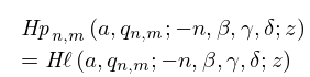
26: 31.5 Solutions Analytic at Three Singularities: Heun Polynomials

… ►

31.5.2 $${\mathrm{𝐻𝑝}}_{n,m}(a,q_{n,m};-n,\beta ,\gamma ,\delta ;z)=H\mathrm{\ell }(a,q_{n,m};-n,\beta ,\gamma ,\delta ;z)$$

ⓘ

Defines:

${\mathrm{𝐻𝑝}}_{n,m}(a,q_{n,m};-n,\beta ,\gamma ,\delta ;z)$: Heun polynomials

Symbols:

$H\mathrm{\ell }(a,q;\alpha ,\beta ,\gamma ,\delta ;z)$: Heun functions, $z$: complex variable, $\gamma$: real or complex parameter, $\delta$: real or complex parameter, $m$: nonnegative integer, $n$: nonnegative integer, $a$: complex parameter, $q$: real or complex parameter and $\beta$: real or complex parameter

Permalink:

http://dlmf.nist.gov/31.5.E2

Encodings:

pMML, png, TeX

See also:

Annotations for §31.5 and Ch.31

…

27: 19.13 Integrals of Elliptic Integrals

… ►

§19.13(i) Integration with Respect to the Modulus

… ►

§19.13(ii) Integration with Respect to the Amplitude

…

28: 1.8 Fourier Series

… ►where $f(x)$ is square-integrable on $[-\pi ,\pi ]$ and $a_n,b_n,c_n$ are given by (1.8.2), (1.8.4). If $g(x)$ is also square-integrable with Fourier coefficients $a_n^{\prime },b_n^{\prime }$ or $c_n^{\prime }$ then … ►Let $f(x)$ be an absolutely integrable function of period $2\pi$, and continuous except at a finite number of points in any bounded interval. … ►

§1.8(iii) Integration and Differentiation

… ►Suppose that $f(x)$ is twice continuously differentiable and $f(x)$ and $\left|f^{\prime \prime }(x)\right|$ are integrable over $(-\mathrm{\infty },\mathrm{\infty })$. …

29: 3.11 Approximation Techniques

… ►

3.11.3 $$m_j={(-1)}^j{ϵ}_n(x_j),$$ $j=0,1,\mathrm{\dots },n+1$.

ⓘ

Defines:

$m_j$: approximation (locally)

Symbols:

${ϵ}_n(x)$: error

Permalink:

http://dlmf.nist.gov/3.11.E3

Encodings:

pMML, png, TeX

See also:

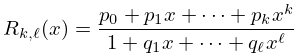
Annotations for §3.11(i), §3.11 and Ch.3

… ►The iterative process converges locally and quadratically (§3.8(i)). … ►They enjoy an orthogonal property with respect to integrals: … ►

3.11.16 $$R_{k,\mathrm{\ell }}(x)=\frac{p_0+p_{1}x+\mathrm{\cdots }+p_k{x}^k}{1+q_{1}x+\mathrm{\cdots }+q_{\mathrm{\ell }}{x}^{\mathrm{\ell }}}$$

ⓘ

Defines:

$R_{k,\mathrm{\ell }}(x)$: rational approximation (locally), $p_k$: coefficients (locally) and $q_{\mathrm{\ell }}$: coefficients (locally)

Referenced by:

§3.11(iii)

Permalink:

http://dlmf.nist.gov/3.11.E16

Encodings:

pMML, png, TeX

See also:

Annotations for §3.11(iii), §3.11 and Ch.3

… ►

3.11.20 $$f(z)=c_0+c_{1}z+c_2{z}^2+\mathrm{\cdots }$$

ⓘ

Defines:

$c_q$: coefficients (locally)

Referenced by:

§3.11(iv)

Permalink:

http://dlmf.nist.gov/3.11.E20

Encodings:

pMML, png, TeX

See also:

Annotations for §3.11(iv), §3.11 and Ch.3

…

30: 1.11 Zeros of Polynomials

… ►

1.11.9

ⓘ

Defines:

$D$: discriminant of $f(z)$ (locally)

Symbols:

$z$: variable, $j$: integer, $k$: integer and $n$: nonnegative integer

Referenced by:

§1.11(ii)

Permalink:

http://dlmf.nist.gov/1.11.E9

Encodings:

pMML, png, TeX

See also:

Annotations for §1.11(ii), §1.11(ii), §1.11 and Ch.1

… ►

1.11.12 $$D=-4p^3-27q^2.$$

ⓘ

Defines:

$D$: discriminant (locally)

Symbols:

$p$ and $q$

A&S Ref:

3.8.1

Permalink:

http://dlmf.nist.gov/1.11.E12

Encodings:

pMML, png, TeX

See also:

Annotations for §1.11(iii), §1.11(iii), §1.11 and Ch.1

… ►

1.11.17 $$D=16p^{4}r-4p^3{q}^2-128p^2{r}^2+144p{q}^{2}r-27q^4+256r^3.$$

ⓘ

Defines:

$D$: discriminant (locally)

Symbols:

$p$ , $q$ and $r$

Permalink:

http://dlmf.nist.gov/1.11.E17

Encodings:

pMML, png, TeX

See also:

Annotations for §1.11(iii), §1.11(iii), §1.11 and Ch.1

… ►Resolvent cubic is $z^3+12z^2+20z+9=0$ with roots ${\theta }_1=-1$, ${\theta }_2=-\frac{1}{2}(11+\sqrt{85})$, ${\theta }_3=-\frac{1}{2}(11-\sqrt{85})$, and $\sqrt{-{\theta }_1}=1$, $\sqrt{-{\theta }_2}=\frac{1}{2}(\sqrt{17}+\sqrt{5})$, $\sqrt{-{\theta }_3}=\frac{1}{2}(\sqrt{17}-\sqrt{5})$. …