limit circle
(0.002 seconds)
1—10 of 100 matching pages
1: 1.18 Linear Second Order Differential Operators and Eigenfunction Expansions
…
►By Weyl’s alternative
equals either 1 (the limit point case) or 2 (the limit circle case), and similarly for .
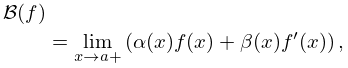
… A boundary value for the end point is a linear form on of the form
►
1.18.71
,
…
►The above results, especially the discussions of deficiency indices and limit point and limit circle boundary conditions, lay the basis for further applications.
…
►The materials developed here follow from the extensions of the Sturm–Liouville theory of second order ODEs as developed by Weyl, to include the limit point and limit circle singular cases.
…
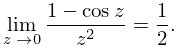
2: 4.31 Special Values and Limits
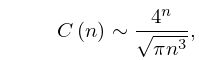
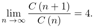
3: 26.5 Lattice Paths: Catalan Numbers
4: 4.17 Special Values and Limits
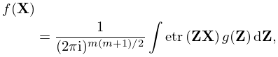
5: 35.2 Laplace Transform
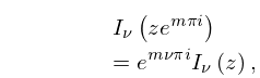
6: 10.34 Analytic Continuation
…
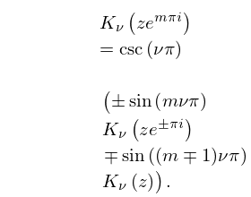
►
10.34.1
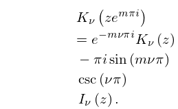
►
10.34.2
…
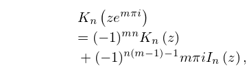
►
10.34.4
►If , then limiting values are taken in (10.34.2) and (10.34.4):
►
10.34.5
…
7: 26.10 Integer Partitions: Other Restrictions
8: 19.20 Special Cases
9: 2.10 Sums and Sequences
…
►(5.11.7) shows that the integrals around the large quarter circles vanish as .
…
►
(b´)
…
►The singularities of on the unit circle are branch points at .
To match the limiting behavior of at these points we set
…
►For uniform expansions when two singularities coalesce on the circle of convergence see Wong and Zhao (2005).
…
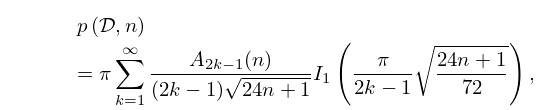
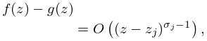
On the circle , the function has a finite number of singularities, and at each singularity , say,
2.10.30
,
where is a positive constant.
