integral%20equation

(0.002 seconds)

21—30 of 30 matching pages

21: Bibliography D

… ►

C. de la Vallée Poussin (1896b) Recherches analytiques sur la théorie des nombres premiers. Deuxième partie. Les fonctions de Dirichlet et les nombres premiers de la forme linéaire

Mx+N

. Ann. Soc. Sci. Bruxelles 20, pp. 281–397 (French).

ⓘ

Notes:: Reprinted in Collected works/Oeuvres scientifiques, Vol. I, pp. 309–425, Académie Royale de Belgique, Brussels, 2000.
External Links:: MathReview, ZentralBlatt
Referenced by:: §25.10(i), §27.11, §27.2(i).
Encodings:: BibTeX

… ►

A. Decarreau, M.-Cl. Dumont-Lepage, P. Maroni, A. Robert, and A. Ronveaux (1978a) Formes canoniques des équations confluentes de l’équation de Heun. Ann. Soc. Sci. Bruxelles Sér. I 92 (1-2), pp. 53–78.

ⓘ

External Links:: MathReview (A. E. Danese), ZentralBlatt
Referenced by:: §31.12.
Encodings:: BibTeX

►

A. Decarreau, P. Maroni, and A. Robert (1978b) Sur les équations confluentes de l’équation de Heun. Ann. Soc. Sci. Bruxelles Sér. I 92 (3), pp. 151–189.

ⓘ

External Links:: ISSN 0037-959X, MathReview, ZentralBlatt
Referenced by:: §31.12.
Encodings:: BibTeX

… ►

B. Döring (1966) Complex zeros of cylinder functions. Math. Comp. 20 (94), pp. 215–222.

ⓘ

Notes:: For a numerical error in one of the zeros see Amos (1985).
External Links:: ISSN 0025-5718, FullText, MathReview, ZentralBlatt
Referenced by:: 2nd item.
Encodings:: BibTeX

… ►

T. M. Dunster (1989) Uniform asymptotic expansions for Whittaker’s confluent hypergeometric functions. SIAM J. Math. Anal. 20 (3), pp. 744–760.

ⓘ

Notes:: (This reference has several typographical errors.)
External Links:: ISSN 0036-1410, Document, MathReview (F. W. J. Olver), ZentralBlatt
Referenced by:: §13.21(ii), §13.21(iii), §13.21(iv).
Encodings:: BibTeX

…

22: 12.10 Uniform Asymptotic Expansions for Large Parameter

… ►

12.10.33

\mathsf{A}_{s+1}(\tau)=-4\tau^{2}(\tau+1)^{2}\frac{\mathrm{d}}{\mathrm{d}\tau}% \mathsf{A}_{s}(\tau)-\frac{1}{4}\int_{0}^{\tau}\left(20u^{2}+20u+3\right)% \mathsf{A}_{s}(u)\,\mathrm{d}u,

s=0,1,2,\dots

ⓘ

Defines:: $\mathsf{A}_{s}(\tau)$ : coefficients (locally)
Symbols:: $\frac{\mathrm{d}\NVar{f}}{\mathrm{d}\NVar{x}}$ : derivative of $f$ with respect to $x$ , $\,\mathrm{d}\NVar{x}$ : differential of $x$ , $\int$ : integral, $s$ : nonnegative integer and $\tau$
Permalink:: http://dlmf.nist.gov/12.10.E33
Encodings:: pMML, png, TeX
See also:: Annotations for §12.10(vi), §12.10 and Ch.12

… ►

\mathsf{A}_{1}(\tau)=-\tfrac{1}{12}\tau(20\tau^{2}+30\tau+9),

…

23: Bibliography R

… ►

J. Raynal (1979) On the definition and properties of generalized

6

j

symbols. J. Math. Phys. 20 (12), pp. 2398–2415.

ⓘ

External Links:: ISSN 0022-2488, Document, MathReview (S. Saran), ZentralBlatt
Referenced by:: §16.4(iii), §16.4(iii).
Encodings:: BibTeX

… ►

W. H. Reid (1972) Composite approximations to the solutions of the Orr-Sommerfeld equation. Studies in Appl. Math. 51, pp. 341–368.

ⓘ

External Links:: MathReview (E. A. Boyd), ZentralBlatt
Referenced by:: (9.13.25), (9.13.26), (9.13.28), (9.13.29), (9.13.32), (9.13.33), (9.13.34), §9.13(ii), §9.13(ii).
Encodings:: BibTeX

►

W. H. Reid (1974a) Uniform asymptotic approximations to the solutions of the Orr-Sommerfeld equation. I. Plane Couette flow. Studies in Appl. Math. 53, pp. 91–110.

ⓘ

External Links:: MathReview (T. W. Kao), ZentralBlatt
Referenced by:: §2.8(iii).
Encodings:: BibTeX

►

W. H. Reid (1974b) Uniform asymptotic approximations to the solutions of the Orr-Sommerfeld equation. II. The general theory. Studies in Appl. Math. 53, pp. 217–224.

ⓘ

External Links:: MathReview (T. W. Kao), ZentralBlatt
Referenced by:: §2.8(iii).
Encodings:: BibTeX

… ►

È. Ya. Riekstynš (1991) Asymptotics and Bounds of the Roots of Equations (Russian). Zinatne, Riga.

ⓘ

External Links:: ISBN 5-7966-0570-4, MathReview (Guillermo López Lagomasino), ZentralBlatt
Referenced by:: §12.11(ii), §6.13.
Encodings:: BibTeX

…

24: 20.11 Generalizations and Analogs

… ►As in §20.11(ii), the modulus

k

of elliptic integrals (§19.2(ii)), Jacobian elliptic functions (§22.2), and Weierstrass elliptic functions (§23.6(ii)) can be expanded in

q

-series via (20.9.1). … ►The first of equations (20.9.2) can also be written … ►The importance of these combined theta functions is that sets of twelve equations for the theta functions often can be replaced by corresponding sets of three equations of the combined theta functions, plus permutation symmetry. Such sets of twelve equations include derivatives, differential equations, bisection relations, duplication relations, addition formulas (including new ones for theta functions), and pseudo-addition formulas. …

25: 25.11 Hurwitz Zeta Function

… ►

See accompanying text — Figure 25.11.1: Hurwitz zeta function $\zeta\left(x,a\right)$ , $a$ = 0. …8, 1, $-20\leq x\leq 10$ . … Magnify

… ►

25.11.6

\zeta\left(s,a\right)=\frac{1}{a^{s}}\left(\frac{1}{2}+\frac{a}{s-1}\right)-% \frac{s(s+1)}{2}\int_{0}^{\infty}\frac{\widetilde{B}_{2}\left(x\right)-B_{2}}{% (x+a)^{s+2}}\,\mathrm{d}x,

s\neq 1

\Re s>-1

a>0

ⓘ

Symbols:: $B_{\NVar{n}}$ : Bernoulli numbers, $\zeta\left(\NVar{s},\NVar{a}\right)$ : Hurwitz zeta function, $\,\mathrm{d}\NVar{x}$ : differential of $x$ , $\int$ : integral, $\widetilde{B}_{\NVar{n}}\left(\NVar{x}\right)$ : periodic Bernoulli functions, $\Re$ : real part, $x$ : real variable, $a$ : real or complex parameter and $s$ : complex variable
Keywords:: Euler–Maclaurin formula, improper integral
Source:: Apostol (1985a, (25), p. 231)
Referenced by:: Erratum (V1.0.12) for Equations (25.11.6), (25.11.19), and (25.11.20)
Permalink:: http://dlmf.nist.gov/25.11.E6
Encodings:: pMML, png, TeX
Errata (effective with 1.0.12):: Originally the integrand was incorrect because its numerator contained the function $\widetilde{B}_{2}\left(x\right)$ . The correct function is $\frac{\widetilde{B}_{2}\left(x\right)-B_{2}}{2}$ .
Reported 2016-05-08 by Clemens Heuberger
See also:: Annotations for §25.11(iii), §25.11 and Ch.25

… ►

§25.11(vii) Integral Representations

… ►

§25.11(viii) Further Integral Representations

… ►

§25.11(ix) Integrals

…

26: 9.18 Tables

… ►

•

Zhang and Jin (1996, p. 337) tabulates $\operatorname{Ai}\left(x\right)$ , $\operatorname{Ai}'\left(x\right)$ , $\operatorname{Bi}\left(x\right)$ , $\operatorname{Bi}'\left(x\right)$ for $x=0(1)20$ to 8S and for $x=-20(1)0$ to 9D.

… ►

•

Miller (1946) tabulates $a_{k}$ , $\operatorname{Ai}'\left(a_{k}\right)$ , $a^{\prime}_{k}$ , $\operatorname{Ai}\left(a^{\prime}_{k}\right)$ , $k=1(1)50$ ; $b_{k}$ , $\operatorname{Bi}'\left(b_{k}\right)$ , $b^{\prime}_{k}$ , $\operatorname{Bi}\left(b^{\prime}_{k}\right)$ , $k=1(1)20$ . Precision is 8D. Entries for $k=1(1)20$ are reproduced in Abramowitz and Stegun (1964, Chapter 10).

►

•

Sherry (1959) tabulates $a_{k}$ , $\operatorname{Ai}'\left(a_{k}\right)$ , $a^{\prime}_{k}$ , $\operatorname{Ai}\left(a^{\prime}_{k}\right)$ , $k=1(1)50$ ; 20S.

►

•

Zhang and Jin (1996, p. 339) tabulates $a_{k}$ , $\operatorname{Ai}'\left(a_{k}\right)$ , $a^{\prime}_{k}$ , $\operatorname{Ai}\left(a^{\prime}_{k}\right)$ , $b_{k}$ , $\operatorname{Bi}'\left(b_{k}\right)$ , $b^{\prime}_{k}$ , $\operatorname{Bi}\left(b^{\prime}_{k}\right)$ , $k=1(1)20$ ; 8D.

… ►

§9.18(v) Integrals

…

27: Bibliography P

… ►

P. Painlevé (1906) Sur les équations différentielles du second ordre à points critiques fixès. C.R. Acad. Sc. Paris 143, pp. 1111–1117.

ⓘ

External Links:: ZentralBlatt
Referenced by:: §32.2(iv).
Encodings:: BibTeX

… ►

R. B. Paris (1992a) Smoothing of the Stokes phenomenon for high-order differential equations. Proc. Roy. Soc. London Ser. A 436, pp. 165–186.

ⓘ

External Links:: ISSN 0962-8444, FullText, MathReview (F. W. J. Olver), ZentralBlatt
Referenced by:: §2.11(v).
Encodings:: BibTeX

… ►

R. Piessens (1982) Automatic computation of Bessel function integrals. Comput. Phys. Comm. 25 (3), pp. 289–295.

ⓘ

Notes:: Double-precision Fortran, maximum accuracy 20S.
External Links:: ISSN 0010-4655, Document, Code
Referenced by:: 6th item.
Encodings:: BibTeX

… ►

G. Pólya (1949) Remarks on computing the probability integral in one and two dimensions. In Proceedings of the Berkeley Symposium on Mathematical Statistics and Probability, 1945, 1946, pp. 63–78.

ⓘ

External Links:: MathReview (L. A. Aroian), ZentralBlatt
Referenced by:: (7.8.8), §7.8, Erratum (V1.0.17) for Equation (7.8.8).
Encodings:: BibTeX

… ►

W. H. Press and S. A. Teukolsky (1990) Elliptic integrals. Computers in Physics 4 (1), pp. 92–96.

ⓘ

Referenced by:: 2nd item.
Encodings:: BibTeX

…

28: 25.12 Polylogarithms

… ►The remainder of the equations in this subsection apply to principal branches. … ►The right-hand side is called Clausen’s integral. … ►

Integral Representation

… ►The Fermi–Dirac and Bose–Einstein integrals are defined by … ►In terms of polylogarithms …

29: 19.36 Methods of Computation

… ►Legendre’s integrals can be computed from symmetric integrals by using the relations in §19.25(i). … ►Complete cases of Legendre’s integrals and symmetric integrals can be computed with quadratic convergence by the AGM method (including Bartky transformations), using the equations in §19.8(i) and §19.22(ii), respectively. … ►For computation of Legendre’s integral of the third kind, see Abramowitz and Stegun (1964, §§17.7 and 17.8, Examples 15, 17, 19, and 20). … ►Numerical quadrature is slower than most methods for the standard integrals but can be useful for elliptic integrals that have complicated representations in terms of standard integrals. … ►

30: 14.30 Spherical and Spheroidal Harmonics

… ►

14.30.8

\int_{0}^{2\pi}\!\!\int_{0}^{\pi}\overline{Y_{{l_{1}},{m_{1}}}\left(\theta,% \phi\right)}Y_{{l_{2}},{m_{2}}}\left(\theta,\phi\right)\sin\theta\,\mathrm{d}% \theta\,\mathrm{d}\phi=\delta_{l_{1},l_{2}}\delta_{m_{1},m_{2}}.

ⓘ

Symbols:: $\delta_{\NVar{j},\NVar{k}}$ : Kronecker delta, $\pi$ : the ratio of the circumference of a circle to its diameter, $\overline{\NVar{z}}$ : complex conjugate, $\,\mathrm{d}\NVar{x}$ : differential of $x$ , $\int$ : integral, $\sin\NVar{z}$ : sine function, $Y_{{\NVar{l}},{\NVar{m}}}\left(\NVar{\theta},\NVar{\phi}\right)$ : spherical harmonic, $m$ : integer and $l$ : nonnegative integer
Referenced by:: §14.30(ii)
Permalink:: http://dlmf.nist.gov/14.30.E8
Encodings:: pMML, png, TeX
Notational Change (effective with 1.0.19):: As a notational clarification, the first spherical harmonic in the integral over $\theta$ been explicity marked up as a complex conjugate.
See also:: Annotations for §14.30(ii), §14.30(ii), §14.30 and Ch.14

►See also (34.3.22), and for further related integrals see Askey et al. (1986). … ►As an example, Laplace’s equation

\nabla^{2}W=0

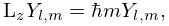
in spherical coordinates (§1.5(ii)): … ►In the quantization of angular momentum the spherical harmonics

Y_{{l},{m}}\left(\theta,\phi\right)

are normalized solutions of the eigenvalue equations … ►

14.30.11_5

\mathrm{L}_{z}Y_{{l},{m}}=\hbar mY_{{l},{m}},

m=-l,-1+1,\dots,0,\dots,l-1,l

ⓘ

Symbols:: $Y_{{\NVar{l}},{\NVar{m}}}\left(\NVar{\theta},\NVar{\phi}\right)$ : spherical harmonic, $m$ : integer, $l$ : nonnegative integer and $\mathrm{L}_{z}$ : $z$ component of the angular momentum operator
Referenced by:: §14.30(iv), Erratum (V1.1.0) for Additions
Permalink:: http://dlmf.nist.gov/14.30.E11_5
Encodings:: pMML, png, TeX
Addition (effective with 1.1.0):: This equation was added.
See also:: Annotations for §14.30(iv), §14.30 and Ch.14

…