differential%20equation

SearchAdvancedHelp

(0.002 seconds)

21—28 of 28 matching pages

21: Bibliography N

… ►

On an integral transform involving a class of Mathieu functions. SIAM J. Math. Anal. 20 (6), pp. 1500–1513.

ⓘ

External Links:

ISSN 0036-1410, Document, MathReview (K. C. Gupta), ZentralBlatt

Referenced by:

§28.26(ii).

Encodings:

BibTeX

… ►

Reduction and evaluation of elliptic integrals. Math. Comp. 20 (94), pp. 223–231.

ⓘ

External Links:

FullText, MathReview (I. A. Stegun), ZentralBlatt

Referenced by:

§19.37(iv).

Encodings:

BibTeX

… ►

Uniform Asymptotic Approximations of Solutions of Second-order Linear Differential Equations, with a Coalescing Simple Turning Point and Simple Pole. Ph.D. Thesis, University of Maryland, College Park, MD.

ⓘ

Referenced by:

§2.8(vi).

Encodings:

BibTeX

… ►

A separating surface for the Painlevé differential equation $x^{\prime \prime }=x^2-t$ . J. Math. Anal. Appl. 193 (3), pp. 817–831.

ⓘ

External Links:

ISSN 0022-247X, Document, MathReview (W. S. Loud), ZentralBlatt

Referenced by:

§32.17.

Encodings:

BibTeX

… ►

Tables of Generalized Airy Functions for the Asymptotic Solution of the Differential Equations $ϵ{(p{y}^{\prime })}^{\prime }+(q+ϵr)y=f$ . Pergamon Press, Oxford.

ⓘ

Notes:

D. E. Brown, translator.

External Links:

MathReview, ZentralBlatt

Referenced by:

4th item.

Encodings:

BibTeX

…

22: 25.11 Hurwitz Zeta Function

… ►

►►

Figure 25.11.1: Hurwitz zeta function $\zeta (x,a)$, $a$ = 0. …8, 1, $-20\le x\le 10$. … Magnify

… ►

25.11.6 $$\zeta (s,a)=\frac{1}{a^s}\left(\frac{1}{2}+\frac{a}{s-1}\right)-\frac{s(s+1)}{2}{\int }_0^{\mathrm{\infty }}\frac{{\tilde{B}}_2\left(x\right)-B_2}{{(x+a)}^{s+2}}dx,$$ $s\ne 1$, $\mathrm{\Re }s>-1$, $a>0$.

ⓘ

Symbols:

$B_n$: Bernoulli numbers, $\zeta (s,a)$: Hurwitz zeta function, $dx$: differential of $x$ , $\int$: integral, ${\tilde{B}}_n\left(x\right)$: periodic Bernoulli functions, $\mathrm{\Re }$: real part, $x$: real variable, $a$: real or complex parameter and $s$: complex variable

Keywords:

Euler–Maclaurin formula, improper integral

Source:

Apostol (1985a, (25), p. 231)

Referenced by:

Erratum (V1.0.12) for Equations (25.11.6), (25.11.19), and (25.11.20)

Permalink:

http://dlmf.nist.gov/25.11.E6

Encodings:

pMML, png, TeX

Errata (effective with 1.0.12):

Originally the integrand was incorrect because its numerator contained the function ${\tilde{B}}_2\left(x\right)$. The correct function is $\frac{{\tilde{B}}_2\left(x\right)-B_2}{2}$.

Reported 2016-05-08 by Clemens Heuberger

See also:

Annotations for §25.11(iii), §25.11 and Ch.25

… ►

25.11.17 $$\frac{\partial }{\partial a}\zeta (s,a)=-s\zeta (s+1,a),$$ $s\ne 0,1$; $\mathrm{\Re }a>0$.

ⓘ

Symbols:

$\zeta (s,a)$: Hurwitz zeta function, $\frac{\partial f}{\partial x}$: partial derivative of $f$ with respect to $x$ , $\partial x$: partial differential of $x$ , $\mathrm{\Re }$: real part, $a$: real or complex parameter and $s$: complex variable

Keywords:

derivative

Proof sketch:

Derivable by differentiating (25.11.1) with respect to $a$.

Referenced by:

(25.11.10)

Permalink:

http://dlmf.nist.gov/25.11.E17

Encodings:

pMML, png, TeX

See also:

Annotations for §25.11(vi), §25.11(vi), §25.11 and Ch.25

… ►

25.11.19 $${\zeta }^{\prime }(s,a)=-\frac{\ln a}{a^s}\left(\frac{1}{2}+\frac{a}{s-1}\right)-\frac{a^{1-s}}{{(s-1)}^2}+\frac{s(s+1)}{2}{\int }_0^{\mathrm{\infty }}\frac{({\tilde{B}}_2\left(x\right)-B_2)\ln \left(x+a\right)}{{(x+a)}^{s+2}}dx-\frac{(2s+1)}{2}{\int }_0^{\mathrm{\infty }}\frac{{\tilde{B}}_2\left(x\right)-B_2}{{(x+a)}^{s+2}}dx,$$ $\mathrm{\Re }s>-1$, $s\ne 1$, $a>0$.

ⓘ

Symbols:

$B_n$: Bernoulli numbers, $\zeta (s,a)$: Hurwitz zeta function, $dx$: differential of $x$ , $\int$: integral, $\ln z$: principal branch of logarithm function, ${\tilde{B}}_n\left(x\right)$: periodic Bernoulli functions, $\mathrm{\Re }$: real part, $x$: real variable, $a$: real or complex parameter, $s$: complex variable and $k$: integer

Keywords:

derivative

Source:

Apostol (1985a, fourth equation, p. 231); with $k=1$, ${\phi }_2(x)=\frac{1}{2}({\tilde{B}}_2\left(x\right)-B_2)$

Referenced by:

Erratum (V1.0.12) for Equations (25.11.6), (25.11.19), and (25.11.20)

Permalink:

http://dlmf.nist.gov/25.11.E19

Encodings:

pMML, png, TeX

Errata (effective with 1.0.12):

Originally both integrands were incorrect because their numerators contained the function ${\tilde{B}}_2\left(x\right)$. The correct function is $\frac{{\tilde{B}}_2\left(x\right)-B_2}{2}$.

Reported 2016-06-27 by Gergő Nemes

See also:

Annotations for §25.11(vi), §25.11(vi), §25.11 and Ch.25

►

25.11.20 $${(-1)}^k{\zeta }^{(k)}(s,a)=\frac{{(\ln a)}^k}{a^s}\left(\frac{1}{2}+\frac{a}{s-1}\right)+k!a^{1-s}\sum _{r=0}^{k-1}\frac{{(\ln a)}^r}{r!{(s-1)}^{k-r+1}}-\frac{s(s+1)}{2}{\int }_0^{\mathrm{\infty }}\frac{({\tilde{B}}_2\left(x\right)-B_2){(\ln \left(x+a\right))}^k}{{(x+a)}^{s+2}}dx+\frac{k(2s+1)}{2}{\int }_0^{\mathrm{\infty }}\frac{({\tilde{B}}_2\left(x\right)-B_2){(\ln \left(x+a\right))}^{k-1}}{{(x+a)}^{s+2}}dx-\frac{k(k-1)}{2}{\int }_0^{\mathrm{\infty }}\frac{({\tilde{B}}_2\left(x\right)-B_2){(\ln \left(x+a\right))}^{k-2}}{{(x+a)}^{s+2}}dx,$$ $\mathrm{\Re }s>-1$, $s\ne 1$, $a>0$.

ⓘ

Symbols:

$B_n$: Bernoulli numbers, $\zeta (s,a)$: Hurwitz zeta function, $dx$: differential of $x$ , $!$: factorial (as in $n!$), $\int$: integral, $\ln z$: principal branch of logarithm function, ${\tilde{B}}_n\left(x\right)$: periodic Bernoulli functions, $\mathrm{\Re }$: real part, $x$: real variable, $a$: real or complex parameter, $s$: complex variable and $k$: integer

Keywords:

derivative

Source:

Apostol (1985a, fourth equation, p. 231); with ${\phi }_2(x)=\frac{1}{2}({\tilde{B}}_2\left(x\right)-B_2)$

Referenced by:

Erratum (V1.0.12) for Equations (25.11.6), (25.11.19), and (25.11.20)

Permalink:

http://dlmf.nist.gov/25.11.E20

Encodings:

pMML, png, TeX

Errata (effective with 1.0.12):

Originally all three integrands were incorrect because their numerators contained the function ${\tilde{B}}_2\left(x\right)$. The correct function is $\frac{{\tilde{B}}_2\left(x\right)-B_2}{2}$.

Reported 2016-06-27 by Gergő Nemes

See also:

Annotations for §25.11(vi), §25.11(vi), §25.11 and Ch.25

…

23: 20.11 Generalizations and Analogs

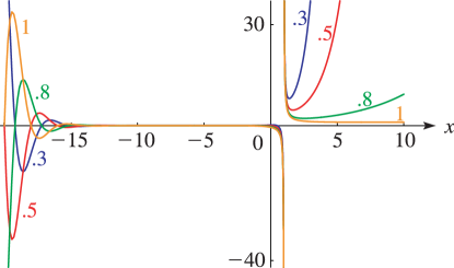
… ►The first of equations (20.9.2) can also be written … ►The importance of these combined theta functions is that sets of twelve equations for the theta functions often can be replaced by corresponding sets of three equations of the combined theta functions, plus permutation symmetry. Such sets of twelve equations include derivatives, differential equations, bisection relations, duplication relations, addition formulas (including new ones for theta functions), and pseudo-addition formulas. …

24: 9.18 Tables

… ►

Zhang and Jin (1996, p. 337) tabulates $\mathrm{Ai}\left(x\right)$, ${\mathrm{Ai}}^{\prime }\left(x\right)$, $\mathrm{Bi}\left(x\right)$, ${\mathrm{Bi}}^{\prime }\left(x\right)$ for $x=0(1)20$ to 8S and for $x=-20(1)0$ to 9D.

… ►

Miller (1946) tabulates $a_k$, ${\mathrm{Ai}}^{\prime }\left(a_k\right)$, $a_k^{\prime }$, $\mathrm{Ai}\left(a_k^{\prime }\right)$, $k=1(1)50$; $b_k$, ${\mathrm{Bi}}^{\prime }\left(b_k\right)$, $b_k^{\prime }$, $\mathrm{Bi}\left(b_k^{\prime }\right)$, $k=1(1)20$. Precision is 8D. Entries for $k=1(1)20$ are reproduced in Abramowitz and Stegun (1964, Chapter 10).

►

Sherry (1959) tabulates $a_k$, ${\mathrm{Ai}}^{\prime }\left(a_k\right)$, $a_k^{\prime }$, $\mathrm{Ai}\left(a_k^{\prime }\right)$, $k=1(1)50$; 20S.

►

Zhang and Jin (1996, p. 339) tabulates $a_k$, ${\mathrm{Ai}}^{\prime }\left(a_k\right)$, $a_k^{\prime }$, $\mathrm{Ai}\left(a_k^{\prime }\right)$, $b_k$, ${\mathrm{Bi}}^{\prime }\left(b_k\right)$, $b_k^{\prime }$, $\mathrm{Bi}\left(b_k^{\prime }\right)$, $k=1(1)20$; 8D.

… ►

Smirnov (1960) tabulates $U_1(x,\alpha )$, $U_2(x,\alpha )$, defined by (9.13.20), (9.13.21), and also $\partial U_1(x,\alpha )/\partial x$, $\partial U_2(x,\alpha )/\partial x$, for $\alpha =1$, $x=-6(.01)10$ to 5D or 5S, and also for $\alpha =\pm \frac{1}{4}$, $\pm \frac{1}{3}$, $\pm \frac{1}{2}$, $\pm \frac{2}{3}$, $\pm \frac{3}{4}$, $\frac{5}{4}$, $\frac{4}{3}$, $\frac{3}{2}$, $\frac{5}{3}$, $\frac{7}{4}$, 2, $x=0(.01)6$; 4D.

25: 25.12 Polylogarithms

… ►

25.12.2 $${\mathrm{Li}}_2\left(z\right)=-{\int }_0^z{t}^{-1}\ln \left(1-t\right)dt,$$ $z\in ℂ\setminus (1,\mathrm{\infty })$.

ⓘ

Symbols:

$ℂ$: complex plane, $dx$: differential of $x$ , ${\mathrm{Li}}_2\left(z\right)$: dilogarithm, $\in$: element of, $\int$: integral, $\ln z$: principal branch of logarithm function, $(a,b)$: open interval, $\setminus$: set subtraction, $x$: real variable and $z$: complex variable

Keywords:

definite integral, integral representation

Source:

Maximon (2003, (2.1), p. 2807)

A&S Ref:

27.7.1 (is a modified form with $z=1-x$)

Referenced by:

§25.12(i)

Permalink:

http://dlmf.nist.gov/25.12.E2

Encodings:

pMML, png, TeX

See also:

Annotations for §25.12(i), §25.12 and Ch.25

… ►The remainder of the equations in this subsection apply to principal branches. … ►

25.12.9 $$\sum _{n=1}^{\mathrm{\infty }}\frac{\sin \left(n\theta \right)}{n^2}=-{\int }_0^{\theta }\ln \left(2\sin \left(\frac{1}{2}x\right)\right)dx.$$

ⓘ

Symbols:

$dx$: differential of $x$ , $\int$: integral, $\ln z$: principal branch of logarithm function, $\sin z$: sine function, $n$: nonnegative integer, $x$: real variable and $\theta$: phase

Keywords:

definite integral, infinite series

Source:

Maximon (2003, (8.7), (8.8), p. 2813)

A&S Ref:

27.8.6 (integration of first series)

Referenced by:

1st item

Permalink:

http://dlmf.nist.gov/25.12.E9

Encodings:

pMML, png, TeX

See also:

Annotations for §25.12(i), §25.12 and Ch.25

… ►

►►

Figure 25.12.1: Dilogarithm function ${\mathrm{Li}}_2\left(x\right)$, Magnify

►

►

►

Figure 25.12.2: Absolute value of the dilogarithm function $\left|{\mathrm{Li}}_2\left(x+\mathrm{i}y\right)\right|$, $-20\le x\le 20$, $-20\le y\le 20$. … Magnify 3D Help

…

26: Bibliography F

… ►

Computation of complex Airy functions and their zeros using asymptotics and the differential equation. ACM Trans. Math. Software 30 (4), pp. 471–490.

ⓘ

External Links:

ISSN 0098-3500, Document, MathReview, ZentralBlatt

Referenced by:

§9.17(ii), §9.17(v), §9.8(iv).

Encodings:

BibTeX

… ►

ⓘ

Notes:

The “Freely Distributable LIBM” package provides implementations of standard elementary functions plus a few higher functions, e.g. gamma. Double precision, maximum accuracy 20S. Developed by Sun Microsystems.

External Links:

GAMS (package FDLIBM)

Referenced by:

§ ‣ Software Cross Index, § ‣ Software Cross Index.

Encodings:

BibTeX

… ►

Sur certaines sommes des intégral-cosinus. Bull. Soc. Math. Phys. Serbie 12, pp. 13–20 (French).

ⓘ

External Links:

MathReview (L. Carlitz), ZentralBlatt

Referenced by:

§6.15.

Encodings:

BibTeX

… ►

Tables of Elliptic Integrals of the First, Second, and Third Kind. Technical report Technical Report ARL 64-232, Aerospace Research Laboratories, Wright-Patterson Air Force Base, Ohio.

ⓘ

Notes:

Reviewed in Math. Comp. v. 1919(1965)509. Table erratum: Math. Comp. v. 20 (1966), no. 96, pp. 639-640.

Referenced by:

§19.37(ii), §19.37(ii), §19.37(iii), §19.37(iii), §19.37(iii).

Encodings:

BibTeX

… ►

On weighted polynomial approximation on the whole real axis. Acta Math. Acad. Sci. Hungar. 20, pp. 223–225.

ⓘ

External Links:

ISSN 0001-5954, Document, Link, MathReview (A. K. Varma)

Referenced by:

§18.32.

Encodings:

BibTeX

…

27: 18.39 Applications in the Physical Sciences

… ►The finite system of functions ${\psi }_n$ is orthonormal in $L^2(ℝ,dx)$, see (18.34.7_3). … ►The Schrödinger equation with potential … ►

Other Analytically Solved Schrödinger Equations

… ►Substitution of (18.39.24) into (18.39.23) then gives the ordinary differential equation for the radial wave function $R_{n,l}(r)$, … ►Derivations of (18.39.42) appear in Bethe and Salpeter (1957, pp. 12–20), and Pauling and Wilson (1985, Chapter V and Appendix VII), where the derivations are based on (18.39.36), and is also the notation of Piela (2014, §4.7), typifying the common use of the associated Coulomb–Laguerre polynomials in theoretical quantum chemistry. …

28: 14.30 Spherical and Spheroidal Harmonics

… ►As an example, Laplace’s equation ${\nabla }^{2}W=0$ in spherical coordinates (§1.5(ii)): ►

14.30.10 $$\frac{1}{{\rho }^2}\frac{\partial }{\partial \rho }\left({\rho }^2\frac{\partial W}{\partial \rho }\right)+\frac{1}{{\rho }^2\sin \theta }\frac{\partial }{\partial \theta }\left(\sin \theta \frac{\partial W}{\partial \theta }\right)+\frac{1}{{\rho }^2{\sin }^2\theta }\frac{{\partial }^{2}W}{{\partial \varphi }^2}=0,$$

ⓘ

Symbols:

$\frac{\partial f}{\partial x}$: partial derivative of $f$ with respect to $x$ , $\partial x$: partial differential of $x$ , $\sin z$: sine function and $W(\rho ,\theta ,\varphi )$: solution

Permalink:

http://dlmf.nist.gov/14.30.E10

Encodings:

pMML, png, TeX

See also:

Annotations for §14.30(iv), §14.30 and Ch.14

… ►In the quantization of angular momentum the spherical harmonics $Y_{l,m}(\theta ,\varphi )$ are normalized solutions of the eigenvalue equations … ►

14.30.12 $$L^2=-{\mathrm{\hslash }}^2\left(\frac{1}{\sin \theta }\frac{\partial }{\partial \theta }\left(\sin \theta \frac{\partial }{\partial \theta }\right)+\frac{1}{{\sin }^2\theta }\frac{{\partial }^2}{{\partial \varphi }^2}\right),$$

ⓘ

Defines:

$L$: angular momentum operator (locally)

Symbols:

$\frac{\partial f}{\partial x}$: partial derivative of $f$ with respect to $x$ , $\partial x$: partial differential of $x$ and $\sin z$: sine function

Referenced by:

§18.39(ii)

Permalink:

http://dlmf.nist.gov/14.30.E12

Encodings:

pMML, png, TeX

See also:

Annotations for §14.30(iv), §14.30 and Ch.14

… ►

14.30.13 $${\mathrm{L}}_z=-\mathrm{i}\mathrm{\hslash }\frac{\partial }{\partial \varphi };$$

ⓘ

Defines:

${\mathrm{L}}_z$: $z$ component of the angular momentum operator (locally)

Symbols:

$\mathrm{i}$: imaginary unit, $\frac{\partial f}{\partial x}$: partial derivative of $f$ with respect to $x$ , $\partial x$: partial differential of $x$ and $z$: complex variable

Referenced by:

§14.30(iv), Erratum (V1.1.0) for Additions

Permalink:

http://dlmf.nist.gov/14.30.E13

Encodings:

pMML, png, TeX

Addition (effective with 1.1.0):

This equation was added.

See also:

Annotations for §14.30(iv), §14.30 and Ch.14

…