§25.11 Hurwitz Zeta Function
- Keywords:
- Hurwitz zeta function, analytic properties
- Notes:
- See Apostol (1976, Chapter 12), Srivastava and Choi (2001), Miller and Adamchik (1998), and Adamchik and Srivastava (1998).
- Referenced by:
- §25.14(i)
- Permalink:
- http://dlmf.nist.gov/25.11
- See also:
- Annotations for Ch.25
Contents
- §25.11(i) Definition
- §25.11(ii) Graphics
- §25.11(iii) Representations by the Euler–Maclaurin Formula
- §25.11(iv) Series Representations
- §25.11(v) Special Values
- §25.11(vi) Derivatives
- §25.11(vii) Integral Representations
- §25.11(viii) Further Integral Representations
- §25.11(ix) Integrals
- §25.11(x) Further Series Representations
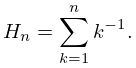
- §25.11(xi) Sums
- §25.11(xii) -Asymptotic Behavior
§25.11(i) Definition
- Keywords:
- Hurwitz zeta function, Riemann zeta function, definition, relations to other functions
- Notes:
- Analytic properties of with respect to follow from (25.11.30).
- Referenced by:
- §8.15
- Permalink:
- http://dlmf.nist.gov/25.11.i
- See also:
- Annotations for §25.11 and Ch.25
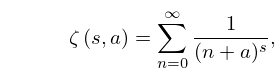
The function was introduced in Hurwitz (1882) and defined by the series expansion
| 25.11.1 | |||
| , . | |||
|
ⓘ
| |||
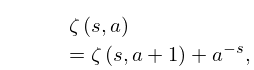
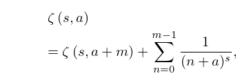
has a meromorphic continuation in the -plane, its only singularity in being a simple pole at with residue . As a function of , with () fixed, is analytic in the half-plane . The Riemann zeta function is a special case:
| 25.11.2 | |||
|
ⓘ
| |||
For most purposes it suffices to restrict because of the following straightforward consequences of (25.11.1):
| 25.11.3 | |||
|
ⓘ
| |||
| 25.11.4 | |||
| . | |||
|
ⓘ
| |||
Most references treat real with .
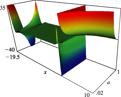
§25.11(ii) Graphics
- Keywords:
- Hurwitz zeta function, graphics
- Notes:
- These graphics were constructed at NIST.
- Permalink:
- http://dlmf.nist.gov/25.11.ii
- See also:
- Annotations for §25.11 and Ch.25
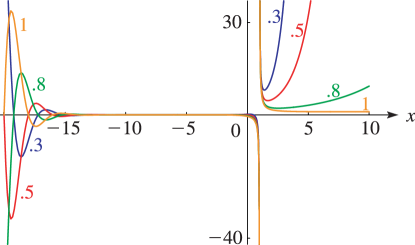
- Symbols:
- : Hurwitz zeta function, : real variable and : real or complex parameter
- Permalink:
- http://dlmf.nist.gov/25.11.F1
- Encodings:
- pdf, png
- See also:
- Annotations for §25.11(ii), §25.11 and Ch.25
- Symbols:
- : Hurwitz zeta function, : real variable and : real or complex parameter
- Permalink:
- http://dlmf.nist.gov/25.11.F2
- Encodings:
- Vizualization, pdf, png
- See also:
- Annotations for §25.11(ii), §25.11 and Ch.25
§25.11(iii) Representations by the Euler–Maclaurin Formula
- Keywords:
- Hurwitz zeta function, representations by Euler–Maclaurin formula
- Permalink:
- http://dlmf.nist.gov/25.11.iii
- See also:
- Annotations for §25.11 and Ch.25
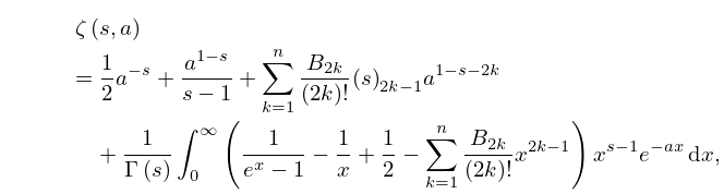
| 25.11.5 | |||
| , , , . | |||
|
ⓘ
| |||
| 25.11.6 | |||
| , , . | |||
|
ⓘ
| |||
| 25.11.7 | |||
| , , , . | |||
|
ⓘ
| |||
For see §24.2(iii).
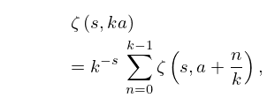
§25.11(iv) Series Representations
- Keywords:
- Hurwitz zeta function, series representations
- Notes:
- See Srivastava and Choi (2001) and Apostol (1976, Section 12.7).
- Referenced by:
- Erratum (V1.0.5) for References
- Permalink:
- http://dlmf.nist.gov/25.11.iv
- Addition (effective with 1.0.5):
- The reference to Coffey (2008) has been added at the end of this subsection.
- See also:
- Annotations for §25.11 and Ch.25
| 25.11.8 | |||
| , , . | |||
|
ⓘ
| |||
| 25.11.9 | |||
| if ; if . | |||
|
ⓘ
| |||
| 25.11.10 | |||
| , . | |||
|
ⓘ
| |||
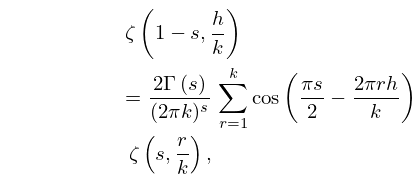
§25.11(v) Special Values
- Keywords:
- Hurwitz zeta function, special values
- Permalink:
- http://dlmf.nist.gov/25.11.v
- See also:
- Annotations for §25.11 and Ch.25
Throughout this subsection .
| 25.11.11 | |||
| . | |||
|
ⓘ
| |||
| 25.11.12 | |||
| . | |||
|
ⓘ
| |||
| 25.11.13 | |||
|
ⓘ
| |||
| 25.11.14 | |||
| . | |||
|
ⓘ
| |||
| 25.11.15 | |||
| , . | |||
|
ⓘ
| |||
| 25.11.16 | |||
| ; integers, . | |||
|
ⓘ
| |||
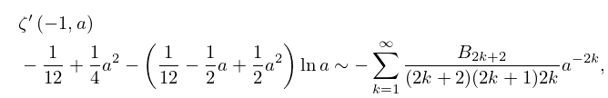
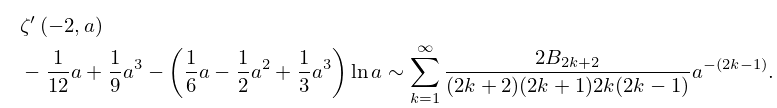
§25.11(vi) Derivatives
- Keywords:
- Hurwitz zeta function, derivatives
- Notes:
- See Apostol (1985a, p. 231) and Miller and Adamchik (1998).
- Permalink:
- http://dlmf.nist.gov/25.11.vi
- See also:
- Annotations for §25.11 and Ch.25
-Derivative
- See also:
- Annotations for §25.11(vi), §25.11 and Ch.25
| 25.11.17 | |||
| ; . | |||
|
ⓘ
| |||
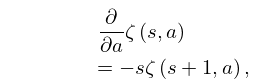
-Derivatives
- See also:
- Annotations for §25.11(vi), §25.11 and Ch.25
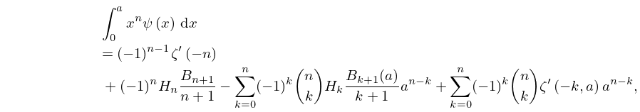
In (25.11.18)–(25.11.24) primes on denote derivatives with respect to . Similarly in §§25.11(viii) and 25.11(xii).
| 25.11.18 | |||
| . | |||
|
ⓘ
| |||
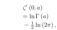
| 25.11.19 | |||
| , , . | |||
|
ⓘ
| |||
| 25.11.20 | |||
| , , . | |||
|
ⓘ
| |||
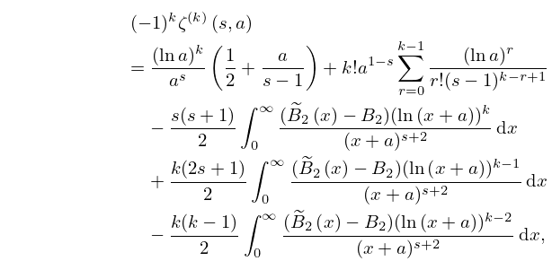
| 25.11.21 | |||
|
ⓘ
| |||
where are integers with and .
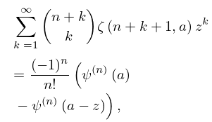
| 25.11.22 | |||
| . | |||
|
ⓘ
| |||
| 25.11.23 | |||
| . | |||
|
ⓘ
| |||
| 25.11.24 | |||
| , . | |||
|
ⓘ
| |||
§25.11(vii) Integral Representations
- Keywords:
- Hurwitz zeta function, integral representations
- Notes:
- See Apostol (1976, Section 12.3).
- Permalink:
- http://dlmf.nist.gov/25.11.vii
- See also:
- Annotations for §25.11 and Ch.25
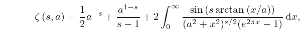
| 25.11.25 | ||||
| , . | ||||
|
ⓘ
| ||||
| 25.11.26 | ||||
| , . | ||||
|
ⓘ
| ||||
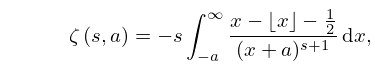
| 25.11.27 | |||
| , , . | |||
|
ⓘ
| |||
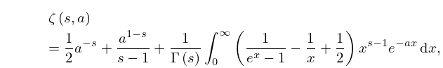
| 25.11.28 | |||
| , , . | |||
|
ⓘ
| |||
| 25.11.29 | |||
| , . | |||
|
ⓘ
| |||
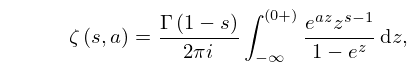
| 25.11.30 | |||
| , , | |||
|
ⓘ
| |||
where the integration contour is a loop around the negative real axis as described for (25.5.20).
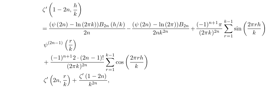
§25.11(viii) Further Integral Representations
- Notes:
- See Adamchik (1998).
- Referenced by:
- §25.11(vi)
- Permalink:
- http://dlmf.nist.gov/25.11.viii
- Addition (effective with 1.1.4):
-
A line of text was added just above (25.11.33) reading
“where are the harmonic numbers:”.
Suggested 2021-08-23 by Gergő Nemes
- See also:
- Annotations for §25.11 and Ch.25
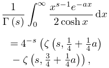
| 25.11.31 | |||
| , . | |||
|
ⓘ
| |||
| 25.11.32 | |||
| , , | |||
|
ⓘ
| |||
where are the harmonic numbers:
| 25.11.33 | |||
|
ⓘ
| |||
| 25.11.34 | |||
| , . | |||
|
ⓘ
| |||
§25.11(ix) Integrals
- Keywords:
- Hurwitz zeta function, integrals
- Permalink:
- http://dlmf.nist.gov/25.11.ix
- See also:
- Annotations for §25.11 and Ch.25
§25.11(x) Further Series Representations
- Keywords:
- Hurwitz zeta function, series representations
- Notes:
- See Apostol (1976, p. 249). For (25.11.35) use (25.11.25) and (25.11.8).
- Referenced by:
- Erratum (V1.1.3) for References
- Permalink:
- http://dlmf.nist.gov/25.11.x
- Removal (effective with 1.1.4):
- The line immediately below (25.11.36) which previously read “where is a Dirichlet character (§27.8). Compare (25.15.1) and (25.15.3).” has been removed because (25.11.36) has been removed.
- Addition (effective with 1.1.4):
- Included mention of (8.15.2) in the last sentence of this subsection.
- Addition (effective with 1.0.23):
- A sentence just below (25.11.36) was added indicating that one should make a comparison with (25.15.1) and (25.15.3).
- See also:
- Annotations for §25.11 and Ch.25
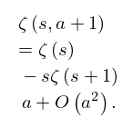
| 25.11.35 | |||
| , ; or , , . | |||
|
ⓘ
| |||
When , (25.11.35) reduces to (25.2.3).
| 25.11.36 | Removed because it is just (25.15.1) combined with (25.15.3). | ||
|
ⓘ
| |||
§25.11(xi) Sums
- Keywords:
- Catalan’s constant, Hurwitz zeta function, Riemann zeta function, sums
- Notes:
- See Adamchik and Srivastava (1998).
- Permalink:
- http://dlmf.nist.gov/25.11.xi
- See also:
- Annotations for §25.11 and Ch.25
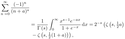
| 25.11.37 | |||
| , . | |||
|
ⓘ
| |||
| 25.11.38 | |||
| , , . | |||
|
ⓘ
| |||
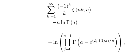
| 25.11.39 | |||
|
ⓘ
| |||
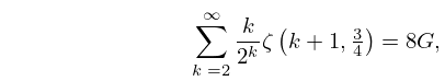
where is Catalan’s constant:
| 25.11.40 | |||
|
ⓘ
| |||
§25.11(xii) -Asymptotic Behavior
- Keywords:
- Hurwitz zeta function, asymptotic expansions for large parameter, derivatives
- Notes:
- See Apostol (1952) and Elizalde (1986).
- Referenced by:
- §25.11(vi)
- Permalink:
- http://dlmf.nist.gov/25.11.xii
- See also:
- Annotations for §25.11 and Ch.25
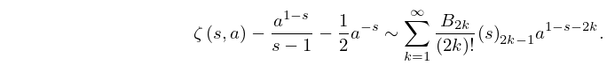
As with fixed,
| 25.11.41 | |||
|
ⓘ
| |||
As with fixed, ,
| 25.11.42 | |||
|
ⓘ
| |||
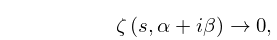
uniformly with respect to bounded nonnegative values of .
As in the sector , with and fixed, we have the asymptotic expansion
| 25.11.43 | |||
|
ⓘ
| |||
Similarly, as in the sector ,
| 25.11.44 | |||
|
ⓘ
| |||
and
| 25.11.45 | |||
|
ⓘ
| |||
For the more general case , , see Elizalde (1986).
