confluent form

SearchAdvancedHelp

(0.002 seconds)

21—30 of 41 matching pages

21: 13.29 Methods of Computation

… ►However, this accuracy can be increased considerably by use of the exponentially-improved forms of expansion supplied by the combination of (13.7.10) and (13.7.11), or by use of the hyperasymptotic expansions given in Olde Daalhuis and Olver (1995a). … ►For $M(a,b,z)$ and $M_{\kappa ,\mu }\left(z\right)$ this means that in the sector $|\mathrm{ph}z|\le \pi$ we may integrate along outward rays from the origin with initial values obtained from (13.2.2) and (13.14.2). ►For $U(a,b,z)$ and $W_{\kappa ,\mu }\left(z\right)$ we may integrate along outward rays from the origin in the sectors , with initial values obtained from connection formulas in §13.2(vii), §13.14(vii). … ►The recurrence relations in §§13.3(i) and 13.15(i) can be used to compute the confluent hypergeometric functions in an efficient way. … ►In Colman et al. (2011) an algorithm is described that uses expansions in continued fractions for high-precision computation of $M(n,b,x)$, when $b$ and $x$ are real and $n$ is a positive integer. …

22: 33.2 Definitions and Basic Properties

… ►The function $F_{\mathrm{\ell }}(\eta ,\rho )$ is recessive (§2.7(iii)) at $\rho =0$, and is defined by …where $M_{\kappa ,\mu }\left(z\right)$ and $M(a,b,z)$ are defined in §§13.14(i) and 13.2(i), and … ►The normalizing constant $C_{\mathrm{\ell }}\left(\eta \right)$ is always positive, and has the alternative form … ►The functions $H_{\mathrm{\ell }}^{\pm }(\eta ,\rho )$ are defined by …where $W_{\kappa ,\mu }\left(z\right)$, $U(a,b,z)$ are defined in §§13.14(i) and 13.2(i), …

23: 18.34 Bessel Polynomials

… ►

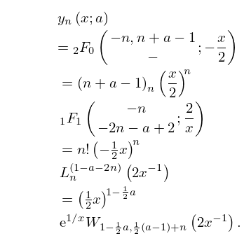
§18.34(i) Definitions and Recurrence Relation

►For the confluent hypergeometric function ${}_1{}^{}F_1^{}$ and the generalized hypergeometric function ${}_2{}^{}F_0^{}$, the Laguerre polynomial $L_n^{(\alpha )}$ and the Whittaker function $W_{\kappa ,\mu }$ see §16.2(ii), §16.2(iv), (18.5.12), and (13.14.3), respectively. ►

18.34.1 $$y_n(x;a)={}_2{}^{}F_0^{}(\genfrac{}{}{0pt}{}{-n,n+a-1}{-};-\frac{x}{2})={\left(n+a-1\right)}_n{\left(\frac{x}{2}\right)}^n{}_1{}^{}F_1^{}(\genfrac{}{}{0pt}{}{-n}{-2n-a+2};\frac{2}{x})=n!{\left(-\frac{1}{2}x\right)}^n{L}_n^{(1-a-2n)}\left(2x^{-1}\right)={\left(\frac{1}{2}x\right)}^{1-\frac{1}{2}a}{\mathrm{e}}^{1/x}{W}_{1-\frac{1}{2}a,\frac{1}{2}(a-1)+n}\left(2x^{-1}\right).$$

ⓘ

Defines:

$y_n(x;a)$: Bessel polynomial

Symbols:

${}_p{}^{}F_q^{}(a_1,\mathrm{\dots },a_p;b_1,\mathrm{\dots },b_q;z)$ or ${}_p{}^{}F_q^{}(\genfrac{}{}{0pt}{}{a_1,\mathrm{\dots },a_p}{b_1,\mathrm{\dots },b_q};z)$: alternatively ${}_p{}^{}F_q^{}(𝐚;𝐛;z)$ or ${}_p{}^{}F_q^{}(\genfrac{}{}{0pt}{}{𝐚}{𝐛};z)$
generalized hypergeometric function, ${}_1{}^{}F_1^{}(a;b;z)$: $=M(a,b,z)$ notation for the Kummer confluent hypergeometric function, $L_n^{(\alpha )}\left(x\right)$: Laguerre (or generalized Laguerre) polynomial, ${\left(a\right)}_n$: Pochhammer’s symbol (or shifted factorial), $W_{\kappa ,\mu }\left(z\right)$: Whittaker confluent hypergeometric function, $\mathrm{e}$: base of natural logarithm, $!$: factorial (as in $n!$), $n$: nonnegative integer and $x$: real variable

Proved:

Grosswald (1978, p.38, Theorem 1); Combine (18.5.12) and items (i), (v), (vii) of the mentioned theorem for $b=2$(proved)

Referenced by:

(18.34.2), (18.34.7_1), §18.34(i), §18.34(i), Erratum (V1.2.0) for Equation (18.34.1)

Permalink:

http://dlmf.nist.gov/18.34.E1

Encodings:

pMML, png, TeX

Addition (effective with 1.2.0):

This equation was updated to include the definition of Bessel polynomials in terms of Laguerre polynomials and the Whittaker confluent hypergeometric function.

See also:

Annotations for §18.34(i), §18.34 and Ch.18

… ►

18.34.7_1 $${\varphi }_n(x;\lambda )={\mathrm{e}}^{-\lambda {\mathrm{e}}^{-x}}{\left(2\lambda {\mathrm{e}}^{-x}\right)}^{\lambda -\frac{1}{2}}{y}_n({\lambda }^{-1}{\mathrm{e}}^x;2-2\lambda )/n!={(-1)}^n{\mathrm{e}}^{-\lambda {\mathrm{e}}^{-x}}{\left(2\lambda {\mathrm{e}}^{-x}\right)}^{\lambda -n-\frac{1}{2}}{L}_n^{(2\lambda -2n-1)}\left(2\lambda {\mathrm{e}}^{-x}\right)={(2\lambda )}^{-\frac{1}{2}}{\mathrm{e}}^{x/2}{W}_{\lambda ,n+\frac{1}{2}-\lambda }\left(2\lambda {\mathrm{e}}^{-x}\right)/n!,$$ $n=0,1,\mathrm{\dots },N=\lceil \lambda -\frac{3}{2}\rceil$, $\lambda >\frac{1}{2}$,

ⓘ

Symbols:

$y_n(x;a)$: Bessel polynomial, $L_n^{(\alpha )}\left(x\right)$: Laguerre (or generalized Laguerre) polynomial, $W_{\kappa ,\mu }\left(z\right)$: Whittaker confluent hypergeometric function, $\lceil x\rceil$: ceiling of $x$ , $\mathrm{e}$: base of natural logarithm, $!$: factorial (as in $n!$), $N$: positive integer, $n$: nonnegative integer and $x$: real variable

Proof sketch:

The second and third equality follow from (18.34.1).

Referenced by:

(18.34.7_2), (18.34.7_3), §18.34(iii), (18.39.17), (18.39.18), §18.39(i), Erratum (V1.2.0) Section 18.34

Permalink:

http://dlmf.nist.gov/18.34.E7_1

Encodings:

pMML, png, TeX

Addition (effective with 1.2.0):

This equation was added.

See also:

Annotations for §18.34(iii), §18.34 and Ch.18

… ►

18.34.8 $$\underset{\alpha \to \mathrm{\infty }}{lim}\frac{P_n^{(\alpha ,a-\alpha -2)}\left(1+\alpha x\right)}{P_n^{(\alpha ,a-\alpha -2)}\left(1\right)}=y_n(x;a).$$

ⓘ

Symbols:

$y_n(x;a)$: Bessel polynomial, $P_n^{(\alpha ,\beta )}\left(x\right)$: Jacobi polynomial, $n$: nonnegative integer and $x$: real variable

Referenced by:

§18.34(iii)

Permalink:

http://dlmf.nist.gov/18.34.E8

Encodings:

pMML, png, TeX

See also:

Annotations for §18.34(iii), §18.34 and Ch.18

…

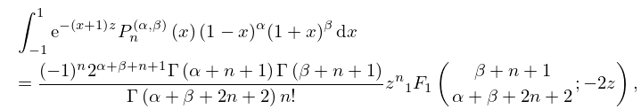
24: 18.17 Integrals

… ►

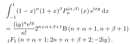
18.17.16 $${\int }_{-1}^1{(1-x)}^{\alpha }{(1+x)}^{\beta }{P}_n^{(\alpha ,\beta )}\left(x\right){\mathrm{e}}^{\mathrm{i}xy}dx=\frac{{(\mathrm{i}y)}^n{\mathrm{e}}^{\mathrm{i}y}}{n!}{2}^{n+\alpha +\beta +1}\mathrm{B}(n+\alpha +1,n+\beta +1){}_1{}^{}F_1^{}(n+\alpha +1;2n+\alpha +\beta +2;-2\mathrm{i}y).$$

ⓘ

Symbols:

$\mathrm{B}(a,b)$: beta function, $P_n^{(\alpha ,\beta )}\left(x\right)$: Jacobi polynomial, ${}_1{}^{}F_1^{}(a;b;z)$: $=M(a,b,z)$ notation for the Kummer confluent hypergeometric function, $dx$: differential of $x$ , $\mathrm{e}$: base of natural logarithm, $!$: factorial (as in $n!$), $\mathrm{i}$: imaginary unit, $\int$: integral, $y$: real variable, $n$: nonnegative integer and $x$: real variable

Referenced by:

§18.17(v), §18.17(vi)

Permalink:

http://dlmf.nist.gov/18.17.E16

Encodings:

pMML, png, TeX

See also:

Annotations for §18.17(v), §18.17(v), §18.17 and Ch.18

►For the beta function $\mathrm{B}(a,b)$ see §5.12, and for the confluent hypergeometric function ${}_1{}^{}F_1^{}$ see (16.2.1) and Chapter 13. … ►

18.17.33 $${\int }_{-1}^1{\mathrm{e}}^{-(x+1)z}{P}_n^{(\alpha ,\beta )}\left(x\right){(1-x)}^{\alpha }{(1+x)}^{\beta }dx=\frac{{(-1)}^n{2}^{\alpha +\beta +n+1}\mathrm{\Gamma }\left(\alpha +n+1\right)\mathrm{\Gamma }\left(\beta +n+1\right)}{\mathrm{\Gamma }\left(\alpha +\beta +2n+2\right)n!}{z}^n{}_1{}^{}F_1^{}(\genfrac{}{}{0pt}{}{\beta +n+1}{\alpha +\beta +2n+2};-2z),$$ $z\in ℂ$.

ⓘ

Symbols:

$\mathrm{\Gamma }\left(z\right)$: gamma function, $P_n^{(\alpha ,\beta )}\left(x\right)$: Jacobi polynomial, ${}_1{}^{}F_1^{}(a;b;z)$: $=M(a,b,z)$ notation for the Kummer confluent hypergeometric function, $ℂ$: complex plane, $dx$: differential of $x$ , $\in$: element of, $\mathrm{e}$: base of natural logarithm, $!$: factorial (as in $n!$), $\int$: integral, $z$: complex variable, $n$: nonnegative integer and $x$: real variable

Referenced by:

§18.17(vi)

Permalink:

http://dlmf.nist.gov/18.17.E33

Encodings:

pMML, png, TeX

See also:

Annotations for §18.17(vi), §18.17(vi), §18.17 and Ch.18

►For the confluent hypergeometric function ${}_1{}^{}F_1^{}$ see (16.2.1) and Chapter 13. … ►Formulas (18.17.45) and (18.17.49) are integrated forms of the linearization formulas (18.18.22) and (18.18.23), respectively. …

25: 33.23 Methods of Computation

… ►

§33.23(i) Methods for the Confluent Hypergeometric Functions

… ►Noble (2004) obtains double-precision accuracy for $W_{-\eta ,\mu }\left(2\rho \right)$ for a wide range of parameters using a combination of recurrence techniques, power-series expansions, and numerical quadrature; compare (33.2.7). …

26: 2.11 Remainder Terms; Stokes Phenomenon

… ►That the change in their forms is discontinuous, even though the function being approximated is analytic, is an example of the Stokes phenomenon. … ►In the transition through $\theta =\pi$, $\mathrm{erfc}\left(\sqrt{\frac{1}{2}\rho }c(\theta )\right)$ changes very rapidly, but smoothly, from one form to the other; compare the graph of its modulus in Figure 2.11.1 in the case $\rho =100$. … ►

2.11.29 $$W_{\kappa ,\mu }\left(z\right)\sim \sum _{n=0}^{\mathrm{\infty }}{a}_n,$$

ⓘ

Symbols:

$W_{\kappa ,\mu }\left(z\right)$: Whittaker confluent hypergeometric function, $\sim$: Poincaré asymptotic expansion and $a_n$: coefficients

Permalink:

http://dlmf.nist.gov/2.11.E29

Encodings:

pMML, png, TeX

See also:

Annotations for §2.11(vi), §2.11 and Ch.2

… ►

2.11.31 $$W_{2.3,0.5}\left(1.0\right)=-\mathrm{0.83299\hspace{0.33em}50268\hspace{0.33em}27526}\mathrm{\cdots }$$

ⓘ

Symbols:

$W_{\kappa ,\mu }\left(z\right)$: Whittaker confluent hypergeometric function

Referenced by:

§2.11(vi)

Permalink:

http://dlmf.nist.gov/2.11.E31

Encodings:

pMML, png, TeX

See also:

Annotations for §2.11(vi), §2.11 and Ch.2

… ►Their extrapolation is based on assumed forms of remainder terms that may not always be appropriate for asymptotic expansions. …

27: 3.10 Continued Fractions

… ►A continued fraction of the form … ►A continued fraction of the form … ►For special functions see §5.10 (gamma function), §7.9 (error function), §8.9 (incomplete gamma functions), §8.17(v) (incomplete beta function), §8.19(vii) (generalized exponential integral), §§10.10 and 10.33 (quotients of Bessel functions), §13.6 (quotients of confluent hypergeometric functions), §13.19 (quotients of Whittaker functions), and §15.7 (quotients of hypergeometric functions). … ►can be written in the form …

28: Bibliography L

… ►

Reduction of Elliptic Integrals to Legendre Normal Form. Technical report Technical Report 97-21, Department of Computer Science, University of Waterloo, Waterloo, Ontario.

ⓘ

Referenced by:

§19.14(ii).

Encodings:

BibTeX

… ►

Asymptotic and numeric study of eigenvalues of the double confluent Heun equation. J. Phys. A 31 (42), pp. 8521–8531.

ⓘ

External Links:

ISSN 0305-4470, Document, MathReview, ZentralBlatt

Referenced by:

§31.13, §31.18.

Encodings:

BibTeX

… ►

New series expansions for the confluent hypergeometric function $M(a,b,z)$ . Appl. Math. Comput. 235, pp. 26–31.

ⓘ

External Links:

ISSN 0096-3003, Document, Link, MathReview Entry, ZentralBlatt

Referenced by:

§13.11, §13.11.

Encodings:

BibTeX

… ►

Algorithms for rational approximations for a confluent hypergeometric function. Utilitas Math. 11, pp. 123–151.

ⓘ

External Links:

MathReview (F. Gotze), ZentralBlatt

Referenced by:

§13.31(iii).

Encodings:

BibTeX

… ►

Adjusted forms of the Fourier coefficient asymptotic expansion and applications in numerical quadrature. Math. Comp. 25 (113), pp. 87–104.

ⓘ

External Links:

FullText, MathReview (J. Bryant), ZentralBlatt

Referenced by:

§2.3(iv).

Encodings:

BibTeX

…

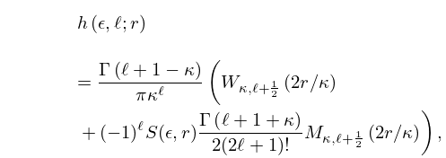
29: 33.14 Definitions and Basic Properties

… ►

§33.14(ii) Regular Solution $f(ϵ,\mathrm{\ell };r)$

… ►where $M_{\kappa ,\mu }\left(z\right)$ and $M(a,b,z)$ are defined in §§13.14(i) and 13.2(i), and … ►For nonzero values of $ϵ$ and $r$ the function $h(ϵ,\mathrm{\ell };r)$ is defined by ►

33.14.7 $$h(ϵ,\mathrm{\ell };r)=\frac{\mathrm{\Gamma }\left(\mathrm{\ell }+1-\kappa \right)}{\pi {\kappa }^{\mathrm{\ell }}}\left(W_{\kappa ,\mathrm{\ell }+\frac{1}{2}}\left(2r/\kappa \right)+{(-1)}^{\mathrm{\ell }}S(ϵ,r)\frac{\mathrm{\Gamma }\left(\mathrm{\ell }+1+\kappa \right)}{2(2\mathrm{\ell }+1)!}{M}_{\kappa ,\mathrm{\ell }+\frac{1}{2}}\left(2r/\kappa \right)\right),$$

ⓘ

Defines:

$h(ϵ,\mathrm{\ell };r)$: irregular Coulomb function

Symbols:

$\mathrm{\Gamma }\left(z\right)$: gamma function, $M_{\kappa ,\mu }\left(z\right)$: Whittaker confluent hypergeometric function, $W_{\kappa ,\mu }\left(z\right)$: Whittaker confluent hypergeometric function, $\pi$: the ratio of the circumference of a circle to its diameter, $!$: factorial (as in $n!$), $\mathrm{\ell }$: nonnegative integer, $r$: real variable, $ϵ$: real parameter, $\kappa$: quantity and $S(ϵ,r)$: function

Referenced by:

§13.18(vi)

Permalink:

http://dlmf.nist.gov/33.14.E7

Encodings:

pMML, png, TeX

See also:

Annotations for §33.14(iii), §33.14 and Ch.33

… ►Note that the functions ${\varphi }_{n,\mathrm{\ell }}$, $n=\mathrm{\ell },\mathrm{\ell }+1,\mathrm{\dots }$, do not form a complete orthonormal system. …

30: 28.8 Asymptotic Expansions for Large $q$

… ►

28.8.6 $${\widehat{C}}_m\sim {\left(\frac{\pi h}{2{(m!)}^2}\right)}^{1/4}{\left(1+\frac{2m+1}{8h}+\frac{m^4+2m^3+263m^2+262m+108}{2048h^2}+\mathrm{\cdots }\right)}^{-1/2},$$

ⓘ

Defines:

${\widehat{C}}_m$: coefficient (locally)

Symbols:

$\sim$: Poincaré asymptotic expansion, $\pi$: the ratio of the circumference of a circle to its diameter, $!$: factorial (as in $n!$), $m$: integer and $h$: parameter

A&S Ref:

20.9.19 (in slightly different form)

Permalink:

http://dlmf.nist.gov/28.8.E6

Encodings:

pMML, png, TeX

See also:

Annotations for §28.8(ii), §28.8 and Ch.28

►

28.8.7 $${\widehat{S}}_m\sim {\left(\frac{\pi h}{2{(m!)}^2}\right)}^{1/4}{\left(1-\frac{2m+1}{8h}+\frac{m^4+2m^3-121m^2-122m-84}{2048h^2}+\mathrm{\cdots }\right)}^{-1/2}.$$

ⓘ

Defines:

${\widehat{S}}_m$: coefficient (locally)

Symbols:

$\sim$: Poincaré asymptotic expansion, $\pi$: the ratio of the circumference of a circle to its diameter, $!$: factorial (as in $n!$), $m$: integer and $h$: parameter

A&S Ref:

20.9.20 (in slightly different form)

Referenced by:

§28.8(ii), Erratum (V1.1.10) for Sections 28.6(i), 28.6(ii), 28.8(i), 28.8(ii)

Permalink:

http://dlmf.nist.gov/28.8.E7

Encodings:

pMML, png, TeX

See also:

Annotations for §28.8(ii), §28.8 and Ch.28

… ►

28.8.9 $$W_m^{\pm }(x)=\frac{{\mathrm{e}}^{\pm 2h\sin x}}{{(\cos x)}^{m+1}}\{\begin{array}{cc}{\left(\cos \left(\frac{1}{2}x+\frac{1}{4}\pi \right)\right)}^{2m+1},\hfill & \\ {\left(\sin \left(\frac{1}{2}x+\frac{1}{4}\pi \right)\right)}^{2m+1},\hfill & \end{array}$$

ⓘ

Defines:

$W_m^{\pm }$: function (locally)

Symbols:

$\pi$: the ratio of the circumference of a circle to its diameter, $\cos z$: cosine function, $\mathrm{e}$: base of natural logarithm, $\sin z$: sine function, $m$: integer, $h$: parameter and $x$: real variable

A&S Ref:

20.9.13 (in slightly different form)

Permalink:

http://dlmf.nist.gov/28.8.E9

Encodings:

pMML, png, TeX

See also:

Annotations for §28.8(iii), §28.8 and Ch.28

… ►

28.8.11 $$P_m(x)\sim 1+\frac{s}{2^{3}h{\cos }^{2}x}+\frac{1}{h^2}\left(\frac{s^4+86s^2+105}{2^{11}{\cos }^{4}x}-\frac{s^4+22s^2+57}{2^{11}{\cos }^{2}x}\right)+\mathrm{\cdots },$$

ⓘ

Defines:

$P_m(x)$ (locally)

Symbols:

$\sim$: Poincaré asymptotic expansion, $\cos z$: cosine function, $m$: integer, $h$: parameter and $x$: real variable

A&S Ref:

20.9.14 (in different form)

Permalink:

http://dlmf.nist.gov/28.8.E11

Encodings:

pMML, png, TeX

See also:

Annotations for §28.8(iii), §28.8 and Ch.28

… ►The approximations are expressed in terms of Whittaker functions $W_{\kappa ,\mu }\left(z\right)$ and $M_{\kappa ,\mu }\left(z\right)$ with $\mu =\frac{1}{4}$; compare §2.8(vi). …