by%20parts

SearchAdvancedHelp

(0.002 seconds)

11—20 of 37 matching pages

11: 26.2 Basic Definitions

… ►For the actual partitions ($\pi$) for $n=1(1)5$ see Table 26.4.1. ►The integers whose sum is $n$ are referred to as the parts in the partition. The example $\{1,1,1,2,4,4\}$ has six parts, three of which equal 1. ►

Table 26.2.1: Partitions $p\left(n\right)$.

► ►►►

$n$	$p\left(n\right)$	$n$	$p\left(n\right)$	$n$	$p\left(n\right)$
…
3	3	20	627	37	21637
…

►

12: Bibliography F

… ►

ⓘ

Notes:

The “Freely Distributable LIBM” package provides implementations of standard elementary functions plus a few higher functions, e.g. gamma. Double precision, maximum accuracy 20S. Developed by Sun Microsystems.

External Links:

GAMS (package FDLIBM)

Referenced by:

§ ‣ Software Cross Index, § ‣ Software Cross Index.

Encodings:

BibTeX

… ►

Sur certaines sommes des intégral-cosinus. Bull. Soc. Math. Phys. Serbie 12, pp. 13–20 (French).

ⓘ

External Links:

MathReview (L. Carlitz), ZentralBlatt

Referenced by:

§6.15.

Encodings:

BibTeX

… ►

Tables of Elliptic Integrals of the First, Second, and Third Kind. Technical report Technical Report ARL 64-232, Aerospace Research Laboratories, Wright-Patterson Air Force Base, Ohio.

ⓘ

Notes:

Reviewed in Math. Comp. v. 1919(1965)509. Table erratum: Math. Comp. v. 20 (1966), no. 96, pp. 639-640.

Referenced by:

§19.37(ii), §19.37(ii), §19.37(iii), §19.37(iii), §19.37(iii).

Encodings:

BibTeX

►

A Table of the Complete Elliptic Integral of the First Kind for Complex Values of the Modulus. Part I. Technical report Technical Report ARL 69-0172, Aerospace Research Laboratories, Office of Aerospace Research, Wright-Patterson Air Force Base, Ohio.

ⓘ

Notes:

Table erratum: Math. Comp. v. 36 (1981), no. 153, p. 318. Part II of this report, with the same date but numbered ARL 69-0173, again puts $k=R\exp (i\theta )$ but with $R$ as parameter and $\theta$ as variable instead of the other way around. Part III, dated May 1970 and numbered ARL 70-0081, contains tables of auxiliary functions to help interpolation.

External Links:

MathReview, ZentralBlatt

Referenced by:

§19.36(ii), §19.37(ii).

Encodings:

BibTeX

… ►

On weighted polynomial approximation on the whole real axis. Acta Math. Acad. Sci. Hungar. 20, pp. 223–225.

ⓘ

External Links:

ISSN 0001-5954, Document, Link, MathReview (A. K. Varma)

Referenced by:

§18.32.

Encodings:

BibTeX

…

13: Bibliography M

… ►

Rational approximations, software and test methods for sine and cosine integrals. Numer. Algorithms 12 (3-4), pp. 259–272.

ⓘ

Notes:

Includes Fortran code, maximum accuracy 20S.

External Links:

ISSN 1017-1398, Document, MathReview, ZentralBlatt

Referenced by:

§6.13, 4th item, §6.21(ii).

Encodings:

BibTeX

… ►

Numerical Methods for Roots of Polynomials. Part I. Studies in Computational Mathematics, Vol. 14, Elsevier, Amsterdam.

ⓘ

External Links:

ISBN 978-0-444-52729-5; 0-444-52729-X, MathReview Entry, ZentralBlatt

Referenced by:

§3.8(iv).

Encodings:

BibTeX

►

Calculation of the modified Bessel functions of the second kind with complex argument. Math. Comp. 20 (95), pp. 407–412.

ⓘ

External Links:

ISSN 0025-5718, FullText, MathReview (H. E. Fettis), ZentralBlatt

Referenced by:

§10.74(iii).

Encodings:

BibTeX

… ►

Hierarchies and logarithmic oscillations in the temporal relaxation patterns of proteins and other complex systems. Proc. Nat. Acad. Sci. U .S. A. 96 (20), pp. 11085–11089.

ⓘ

External Links:

FullText

Referenced by:

§8.24(i).

Encodings:

BibTeX

… ►

The $q$-analogue of the Laguerre polynomials. J. Math. Anal. Appl. 81 (1), pp. 20–47.

ⓘ

External Links:

ISSN 0022-247X, Document, MathReview (R. A. Askey), ZentralBlatt

Referenced by:

§18.27(v).

Encodings:

BibTeX

…

14: 18.40 Methods of Computation

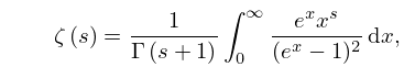
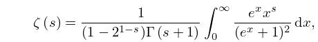
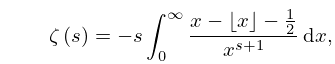
… ►It is now necessary to take the limit $\epsilon \to 0+$ of $F(x^{\prime }+\mathrm{i}\epsilon )$, and the imaginary part is the required Stieltjes–Perron inversion: …The question is then: how is this possible given only $F_N(z)$, rather than $F(z)$ itself? $F_N(z)$ often converges to smooth results for $z$ off the real axis for $\mathrm{\Im }z$ at a distance greater than the pole spacing of the $x_n$, this may then be followed by approximate numerical analytic continuation via fitting to lower order continued fractions (either Padé, see §3.11(iv), or pointwise continued fraction approximants, see Schlessinger (1968, Appendix)), to $F_N(z)$ and evaluating these on the real axis in regions of higher pole density that those of the approximating function. Results of low ($2$ to $3$ decimal digits) precision for $w(x)$ are easily obtained for $N\sim 10$ to $20$. …

15: 26.9 Integer Partitions: Restricted Number and Part Size

§26.9 Integer Partitions: Restricted Number and Part Size

… ► $p_k\left(n\right)$ denotes the number of partitions of $n$ into at most $k$ parts. … … ►Conjugation establishes a one-to-one correspondence between partitions of $n$ into at most $k$ parts and partitions of $n$ into parts with largest part less than or equal to $k$. … ►equivalently, partitions into at most $k$ parts either have exactly $k$ parts, in which case we can subtract one from each part, or they have strictly fewer than $k$ parts. …

16: 25.5 Integral Representations

… ►

25.5.2 $$\zeta \left(s\right)=\frac{1}{\mathrm{\Gamma }\left(s+1\right)}{\int }_0^{\mathrm{\infty }}\frac{{\mathrm{e}}^x{x}^s}{{({\mathrm{e}}^x-1)}^2}dx,$$ $\mathrm{\Re }s>1$.

ⓘ

Symbols:

$\mathrm{\Gamma }\left(z\right)$: gamma function, $\zeta \left(s\right)$: Riemann zeta function, $dx$: differential of $x$ , $\mathrm{e}$: base of natural logarithm, $\int$: integral, $\mathrm{\Re }$: real part, $x$: real variable and $s$: complex variable

Keywords:

improper integral, integral representation

Proof sketch:

Derivable from (25.5.1) by integration by parts.

Permalink:

http://dlmf.nist.gov/25.5.E2

Encodings:

pMML, png, TeX

See also:

Annotations for §25.5(i), §25.5 and Ch.25

… ►

25.5.4 $$\zeta \left(s\right)=\frac{1}{(1-2^{1-s})\mathrm{\Gamma }\left(s+1\right)}{\int }_0^{\mathrm{\infty }}\frac{{\mathrm{e}}^x{x}^s}{{({\mathrm{e}}^x+1)}^2}dx,$$ $\mathrm{\Re }s>0$.

ⓘ

Symbols:

$\mathrm{\Gamma }\left(z\right)$: gamma function, $\zeta \left(s\right)$: Riemann zeta function, $dx$: differential of $x$ , $\mathrm{e}$: base of natural logarithm, $\int$: integral, $\mathrm{\Re }$: real part, $x$: real variable and $s$: complex variable

Keywords:

improper integral, integral representation

Proof sketch:

Derivable from (25.5.3) by integration by parts.

Permalink:

http://dlmf.nist.gov/25.5.E4

Encodings:

pMML, png, TeX

See also:

Annotations for §25.5(i), §25.5 and Ch.25

►

25.5.5 $$\zeta \left(s\right)=-s{\int }_0^{\mathrm{\infty }}\frac{x-\lfloor x\rfloor -\frac{1}{2}}{x^{s+1}}dx,$$ .

ⓘ

Symbols:

$\zeta \left(s\right)$: Riemann zeta function, $dx$: differential of $x$ , $\lfloor x\rfloor$: floor of $x$ , $\int$: integral, $\mathrm{\Re }$: real part, $x$: real variable and $s$: complex variable

Keywords:

improper integral, integral representation

Source:

Titchmarsh (1986b, (2.1.6), p. 15)

Permalink:

http://dlmf.nist.gov/25.5.E5

Encodings:

pMML, png, TeX

See also:

Annotations for §25.5(i), §25.5 and Ch.25

… ►In (25.5.15)–(25.5.19), , $\psi \left(x\right)$ is the digamma function, and $\gamma$ is Euler’s constant (§5.2). (25.5.16) is also valid for , $s\ne 1$. …

17: 6.16 Mathematical Applications

… ►By integration by parts … ►If we assume Riemann’s hypothesis that all nonreal zeros of $\zeta \left(s\right)$ have real part of $\frac{1}{2}$ (§25.10(i)), then … ►

►►

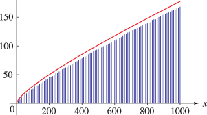
Figure 6.16.2: The logarithmic integral $\mathrm{li}\left(x\right)$, together with vertical bars indicating the value of $\pi (x)$ for $x=10,20,\mathrm{\dots },1000$. Magnify

18: 5.22 Tables

… ►Abramowitz and Stegun (1964, Chapter 6) tabulates $\mathrm{\Gamma }\left(x\right)$, $\ln \mathrm{\Gamma }\left(x\right)$, $\psi \left(x\right)$, and ${\psi }^{\prime }\left(x\right)$ for $x=1(.005)2$ to 10D; ${\psi }^{\prime \prime }\left(x\right)$ and ${\psi }^{(3)}\left(x\right)$ for $x=1(.01)2$ to 10D; $\mathrm{\Gamma }\left(n\right)$, $1/\mathrm{\Gamma }\left(n\right)$, $\mathrm{\Gamma }\left(n+\frac{1}{2}\right)$, $\psi \left(n\right)$, ${\log }_{10}\mathrm{\Gamma }\left(n\right)$, ${\log }_{10}\mathrm{\Gamma }\left(n+\frac{1}{3}\right)$, ${\log }_{10}\mathrm{\Gamma }\left(n+\frac{1}{2}\right)$, and ${\log }_{10}\mathrm{\Gamma }\left(n+\frac{2}{3}\right)$ for $n=1(1)101$ to 8–11S; $\mathrm{\Gamma }\left(n+1\right)$ for $n=100(100)1000$ to 20S. … ►Zhang and Jin (1996, pp. 70, 71, and 73) tabulates the real and imaginary parts of $\mathrm{\Gamma }\left(x+\mathrm{i}y\right)$, $\ln \mathrm{\Gamma }\left(x+\mathrm{i}y\right)$, and $\psi \left(x+\mathrm{i}y\right)$ for $x=0.5,1,5,10$, $y=0(.5)10$ to 8S.

19: Bibliography B

… ►

Pionic atoms. Annual Review of Nuclear and Particle Science 20, pp. 467–508.

ⓘ

External Links:

Document

Referenced by:

§33.22(iv).

Encodings:

BibTeX

… ►

A program for computing the Riemann zeta function for complex argument. Comput. Phys. Comm. 20 (3), pp. 441–445.

ⓘ

Notes:

Double-precision Fortran, maximum accuracy 10S.

External Links:

Document, Code, ZentralBlatt

Referenced by:

1st item.

Encodings:

BibTeX

… ►

Coulomb functions (negative energies). Comput. Phys. Comm. 20 (3), pp. 447–458.

ⓘ

Notes:

Double-precision Fortran code.

External Links:

Document, Code

Referenced by:

1st item, 4th item.

Encodings:

BibTeX

… ►

Some solutions of the problem of forced convection. Philos. Mag. Series 7 20, pp. 322–343.

ⓘ

External Links:

Document, ZentralBlatt

Referenced by:

§10.73(iv).

Encodings:

BibTeX

… ►

Bessel functions and modular relations of higher type and hyperbolic differential equations. Comm. Sém. Math. Univ. Lund [Medd. Lunds Univ. Mat. Sem.] 1952 (Tome Supplementaire), pp. 12–20.

ⓘ

External Links:

MathReview (S. C. van Veen), ZentralBlatt

Referenced by:

§35.5(i).

Encodings:

BibTeX

…

20: 25.12 Polylogarithms

… ►

►►

Figure 25.12.1: Dilogarithm function ${\mathrm{Li}}_2\left(x\right)$, Magnify

►

►

►

Figure 25.12.2: Absolute value of the dilogarithm function $\left|{\mathrm{Li}}_2\left(x+\mathrm{i}y\right)\right|$, $-20\le x\le 20$, $-20\le y\le 20$. … Magnify 3D Help

… ►The series also converges when $|z|=1$, provided that $\mathrm{\Re }s>1$. … ►valid when $\mathrm{\Re }s>0$ and , or $\mathrm{\Re }s>1$ and $z=1$. … ►valid when $\mathrm{\Re }s>0$, $\mathrm{\Im }a>0$ or $\mathrm{\Re }s>1$, $\mathrm{\Im }a=0$. …