alternative forms

(0.001 seconds)

11—20 of 26 matching pages

11: 16.10 Expansions in Series of ${{}_{p}F_{q}}$ Functions

… ►

16.10.1

{{}_{p+r}F_{q+s}}\left({a_{1},\dots,a_{p},c_{1},\dots,c_{r}\atop b_{1},\dots,b% _{q},d_{1},\dots,d_{s}};z\zeta\right)=\sum_{k=0}^{\infty}\frac{{\left(\mathbf{% a}\right)_{k}}{\left(\alpha\right)_{k}}{\left(\beta\right)_{k}}(-z)^{k}}{{% \left(\mathbf{b}\right)_{k}}{\left(\gamma+k\right)_{k}}k!}{{}_{p+2}F_{q+1}}% \left({\alpha+k,\beta+k,a_{1}+k,\dots,a_{p}+k\atop\gamma+2k+1,b_{1}+k,\dots,b_% {q}+k};z\right){{}_{r+2}F_{s+2}}\left({-k,\gamma+k,c_{1},\dots,c_{r}\atop% \alpha,\beta,d_{1},\dots,d_{s}};\zeta\right).

ⓘ

Symbols:: ${{}_{\NVar{p}}F_{\NVar{q}}}\left(\NVar{a_{1},\dots,a_{p}};\NVar{b_{1},\dots,b_% {q}};\NVar{z}\right)$ or ${{}_{\NVar{p}}F_{\NVar{q}}}\left({\NVar{a_{1},\dots,a_{p}}\atop\NVar{b_{1},% \dots,b_{q}}};\NVar{z}\right)$ : alternatively ${{}_{\NVar{p}}F_{\NVar{q}}}\left(\NVar{\mathbf{a}};\NVar{\mathbf{b}};\NVar{z}\right)$ or ${{}_{\NVar{p}}F_{\NVar{q}}}\left({\NVar{\mathbf{a}}\atop\NVar{\mathbf{b}}};% \NVar{z}\right)$
generalized hypergeometric function, ${\left(\NVar{a}\right)_{\NVar{n}}}$ : Pochhammer’s symbol (or shifted factorial), $!$ : factorial (as in $n!$ ), $p$ : nonnegative integer, $q$ : nonnegative integer, $z$ : complex variable, $a,a_{1},\ldots,a_{p}$ : real or complex parameters and $b,b_{1},\ldots,b_{q}$ : real or complex parameters
Permalink:: http://dlmf.nist.gov/16.10.E1
Encodings:: pMML, png, TeX
See also:: Annotations for §16.10 and Ch.16

… ►

16.10.2

{{}_{p+1}F_{p}}\left({a_{1},\dots,a_{p+1}\atop b_{1},\dots,b_{p}};z\zeta\right% )=(1-z)^{-a_{1}}\sum_{k=0}^{\infty}\frac{{\left(a_{1}\right)_{k}}}{k!}{{}_{p+1% }F_{p}}\left({-k,a_{2},\dots,a_{p+1}\atop b_{1},\dots,b_{p}};\zeta\right)\left% (\frac{z}{z-1}\right)^{k}.

ⓘ

Symbols:: ${{}_{\NVar{p}}F_{\NVar{q}}}\left(\NVar{a_{1},\dots,a_{p}};\NVar{b_{1},\dots,b_% {q}};\NVar{z}\right)$ or ${{}_{\NVar{p}}F_{\NVar{q}}}\left({\NVar{a_{1},\dots,a_{p}}\atop\NVar{b_{1},% \dots,b_{q}}};\NVar{z}\right)$ : alternatively ${{}_{\NVar{p}}F_{\NVar{q}}}\left(\NVar{\mathbf{a}};\NVar{\mathbf{b}};\NVar{z}\right)$ or ${{}_{\NVar{p}}F_{\NVar{q}}}\left({\NVar{\mathbf{a}}\atop\NVar{\mathbf{b}}};% \NVar{z}\right)$
generalized hypergeometric function, ${\left(\NVar{a}\right)_{\NVar{n}}}$ : Pochhammer’s symbol (or shifted factorial), $!$ : factorial (as in $n!$ ), $p$ : nonnegative integer, $z$ : complex variable, $a,a_{1},\ldots,a_{p}$ : real or complex parameters and $b,b_{1},\ldots,b_{q}$ : real or complex parameters
Permalink:: http://dlmf.nist.gov/16.10.E2
Encodings:: pMML, png, TeX
See also:: Annotations for §16.10 and Ch.16

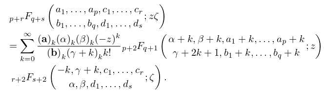
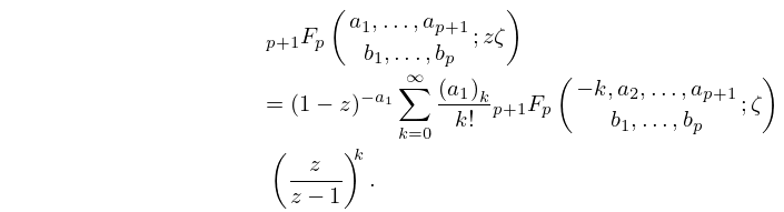
… ►Expansions of the form

\sum_{n=1}^{\infty}(\pm 1)^{n}{{}_{p}F_{p+1}}\left(\mathbf{a};\mathbf{b};-n^{2% }z^{2}\right)

are discussed in Miller (1997), and further series of generalized hypergeometric functions are given in Luke (1969b, Chapter 9), Luke (1975, §§5.10.2 and 5.11), and Prudnikov et al. (1990, §§5.3, 6.8–6.9).

12: 36.5 Stokes Sets

… ►The Stokes set takes different forms for

z=0

z<0

, and

z>0

. … ►Alternatively, when

|X|<X_{2}

…

13: 3.5 Quadrature

… ►Similar results hold for the trapezoidal rule in the form … ►If

f\in C^{2m+2}[a,b]

, then the remainder

E_{n}(f)

in (3.5.2) can be expanded in the form … ►Integrals of the form … ►The integral is written as an alternating series of positive and negative subintegrals that are computed individually; see Longman (1956). … ►For integrals in higher dimensions, Monte Carlo methods are another—often the only—alternative. …

14: 3.10 Continued Fractions

… ►A continued fraction of the form … ►A continued fraction of the form … ►can be written in the form … ►Alternatives to Steed’s algorithm are the Lentz algorithm Lentz (1976) and the modified Lentz algorithm Thompson and Barnett (1986). …

15: 3.6 Linear Difference Equations

… ►Many special functions satisfy second-order recurrence relations, or difference equations, of the form … ►However, there are alternative procedures that do not require

w_{N}

and

w_{N+1}

to be known in advance. … ►The normalizing factor

\Lambda

can be the true value of

w_{0}

divided by its trial value, or

\Lambda

can be chosen to satisfy a known property of the wanted solution of the form … ►Let us assume the normalizing condition is of the form

w_{0}=\lambda

, where

\lambda

is a constant, and then solve the following tridiagonal system of algebraic equations for the unknowns

w_{1}^{(N)},w_{2}^{(N)},\dots,w_{N-1}^{(N)}

; see §3.2(ii). … ►For further information, including a more general form of normalizing condition, other examples, convergence proofs, and error analyses, see Olver (1967a), Olver and Sookne (1972), and Wimp (1984, Chapter 6). …

16: 19.16 Definitions

… ►All elliptic integrals of the form (19.2.3) and many multiple integrals, including (19.23.6) and (19.23.6_5), are special cases of a multivariate hypergeometric function …Before 1969

R_{-a}\left(\mathbf{b};\mathbf{z}\right)

was denoted by

R(a;\mathbf{b};\mathbf{z})

. …

17: 11.9 Lommel Functions

… ►The inhomogeneous Bessel differential equation … ►

11.9.4

a_{k}(\mu,\nu)=\prod_{m=1}^{k}\left((\mu+2m-1)^{2}-\nu^{2}\right)=4^{k}{\left(% \frac{\mu-\nu+1}{2}\right)_{k}}{\left(\frac{\mu+\nu+1}{2}\right)_{k}},

k=0,1,2,\dots

ⓘ

Symbols:: ${\left(\NVar{a}\right)_{\NVar{n}}}$ : Pochhammer’s symbol (or shifted factorial), $\nu$ : real or complex order, $k$ : nonnegative integer and $a_{k}(\mu,\nu)$ : expansion function
Referenced by:: §11.9(iii), Erratum (V1.1.3) for Additions
Permalink:: http://dlmf.nist.gov/11.9.E4
Encodings:: pMML, png, TeX
Addition (effective with 1.1.3):: An alternative Pochhammer symbol representation was added.
See also:: Annotations for §11.9(i), §11.9 and Ch.11

… ►the right-hand side being replaced by its limiting form when

\mu\pm\nu

is an odd negative integer. … ► …

18: 18.33 Polynomials Orthogonal on the Unit Circle

… ►For an alternative and more detailed approach to the recurrence relations, see §18.33(vi). … ►

§18.33(vi) Alternative Set-up with Monic Polynomials

… ►for some weight function

w(z)

(

\geq 0

) then (18.33.17) (see also (18.33.1)) takes the form …

19: 33.14 Definitions and Basic Properties

… ►An alternative formula for

A(\epsilon,\ell)

is … ►Note that the functions

\phi_{n,\ell}

n=\ell,\ell+1,\ldots

, do not form a complete orthonormal system. …

20: 4.13 Lambert $W$ -Function

… ►Alternative notations are

\operatorname{Wp}\left(x\right)

for

W_{0}\left(x\right)

\operatorname{Wm}\left(x\right)

for

W_{-1}\left(x+0\mathrm{i}\right)

, both previously used in this section, the Wright

\omega

-function

\omega\left(z\right)=W\left({\mathrm{e}}^{z}\right)

, which is single-valued, satisfies … ►

4.13.3_1

W_{0}\left(x{\mathrm{e}}^{x}\right)=\begin{cases}x,&-1\leq x,\\ \text{(no simpler form)},&x<-1.\end{cases}

ⓘ

Symbols:: $W\left(\NVar{z}\right)$ : Lambert $W$ -function, $\mathrm{e}$ : base of natural logarithm and $x$ : real variable
Proof sketch:: Take $x=W_{0}\left(t\right)>-1$ , with $t>-{\mathrm{e}}^{-1}$ . Then $W_{0}\left(x{\mathrm{e}}^{x}\right)=W_{0}\left(W_{0}\left(t\right){\mathrm{e}}% ^{W_{0}\left(t\right)}\right)=W_{0}\left(t\right)=x$ .
Referenced by:: §4.13, Erratum (V1.1.7) for Expansion
Permalink:: http://dlmf.nist.gov/4.13.E3_1
Encodings:: pMML, png, TeX
Addition (effective with 1.1.7):: This equation was added.
See also:: Annotations for §4.13 and Ch.4

►

4.13.3_2

W_{\pm 1}\left(x{\mathrm{e}}^{x}\mp 0\mathrm{i}\right)=\begin{cases}\text{(no % simpler form)},&-1\leq x,\\ x,&x<-1.\end{cases}

ⓘ

Symbols:: $W\left(\NVar{z}\right)$ : Lambert $W$ -function, $\mathrm{e}$ : base of natural logarithm, $\mathrm{i}$ : imaginary unit and $x$ : real variable
Proof sketch:: Take $x=W_{1}\left(t-0\mathrm{i}\right)<-1$ , with $-{\mathrm{e}}^{-1}<t<0$ . Then $W_{1}\left(x{\mathrm{e}}^{x}-0\mathrm{i}\right)=W_{1}\left(W_{1}\left(t-0% \mathrm{i}\right){\mathrm{e}}^{W_{1}\left(t-0\mathrm{i}\right)}-0\mathrm{i}% \right)=W_{1}\left(t-0\mathrm{i}\right)=x$ .
Referenced by:: §4.13, Erratum (V1.1.7) for Expansion
Permalink:: http://dlmf.nist.gov/4.13.E3_2
Encodings:: pMML, png, TeX
Addition (effective with 1.1.7):: This equation was added.
See also:: Annotations for §4.13 and Ch.4

…