…
►In (
8.6.10)–(
8.6.12),
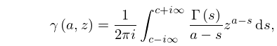
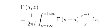
is a real constant and the path of integration is indented (if necessary) so that in the case of (
8.6.10) it separates the poles of the gamma function from the pole at
, in the case of (
8.6.11) it is to the right of all poles, and in the case of (
8.6.12) it separates the poles of the gamma function from the poles at
.
►
8.6.10
, ,
►
8.6.11
,
►
8.6.12
, .
…
►For collections of integral representations of
and
see
Erdélyi et al. (1953b, §9.3),
Oberhettinger (1972, pp. 68–69),
Oberhettinger and Badii (1973, pp. 309–312),
Prudnikov et al. (1992b, §3.10), and
Temme (1996b, pp. 282–283).
…
►For
…
►
is the number of permutations of
with
cycles of length 1,
cycles of length
2,
, and
cycles of length
:
…
is the number of set partitions of
with
subsets of size 1,
subsets of size
2,
, and
subsets of size
:
…For each
all possible values of
are covered.
…
►where the summation is over all nonnegative integers
such that
.
…
…
►Thus
is the permutation
,
,
.
…
►Here
, and
.
…
►A
lattice path is a directed path on the plane integer lattice
.
…
►As an example,
,
,
is a partition of
.
…
►As an example,
is a partition of 13.
…
…
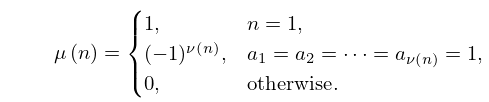
►where
are the distinct prime factors of
, each exponent
is positive, and
is the number of distinct primes dividing
.
…Euclid’s Elements (
Euclid (1908, Book IX, Proposition 20)) gives an elegant proof that there are infinitely many primes.
…
►The
numbers
are relatively prime to
and distinct (mod
).
…It is the special case
of the function
that counts the number of ways of expressing
as the product of
factors, with the order of factors taken into account.
…
►
27.2.12
…
…
►The notation
was introduced in
Lewin (1981) for a function discussed in
Euler (1768) and called the
dilogarithm in
Hill (1828):
…
►Other notations and names for
include
(
Kölbig et al. (1970)), Spence function
(
’t Hooft and Veltman (1979)), and
(
Maximon (2003)).
►In the complex plane
has a branch point at
.
…
►When
,
, (
25.12.1) becomes
…
►When
and
, (
25.12.13) becomes (
25.12.4).
…
