Pochhammer%20integral
(0.002 seconds)
21—30 of 545 matching pages
21: 5.18 -Gamma and -Beta Functions
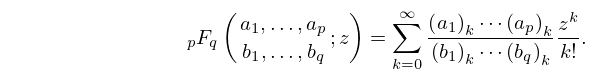
22: 16.2 Definition and Analytic Properties
…
►
16.2.1
…
►
16.2.3
…
►
16.2.4
…
►See §16.5 for the definition of as a contour integral when and none of the is a nonpositive integer.
…
►
16.2.5
…
23: 19.12 Asymptotic Approximations
§19.12 Asymptotic Approximations
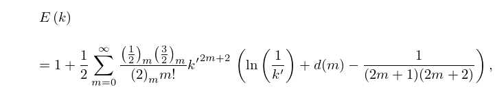
►With denoting the digamma function (§5.2(i)) in this subsection, the asymptotic behavior of and near the singularity at is given by the following convergent series: … ►
19.12.2
,
…
►For the asymptotic behavior of and as and see Kaplan (1948, §2), Van de Vel (1969), and Karp and Sitnik (2007).
…
►Asymptotic approximations for , with different variables, are given in Karp et al. (2007).
…
24: 7.12 Asymptotic Expansions
…
►
§7.12(ii) Fresnel Integrals
►The asymptotic expansions of and are given by (7.5.3), (7.5.4), and … ►They are bounded by times the first neglected terms when . … ►§7.12(iii) Goodwin–Staton Integral
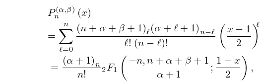
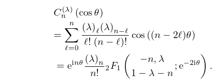
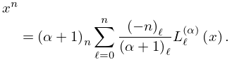
►See Olver (1997b, p. 115) for an expansion of with bounds for the remainder for real and complex values of .25: 18.5 Explicit Representations
26: 13.29 Methods of Computation
…
►
§13.29(iii) Integral Representations
►The integral representations (13.4.1) and (13.4.4) can be used to compute the Kummer functions, and (13.16.1) and (13.16.5) for the Whittaker functions. … ►
13.29.3
…
►
13.29.6
…
►
13.29.7
…
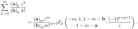
27: 18.18 Sums
…
►Assume also the integrals
and converge.
…
►Assume also converges.
…
►Assume also converges.
…
►For integral representations for products implied by (18.18.8) and (18.18.9) see (18.17.5) and (18.17.6), respectively.
…
►
18.18.19
…
28: 31.11 Expansions in Series of Hypergeometric Functions
…
►Series of Type II (§31.11(iv)) are expansions in orthogonal polynomials, which are useful in calculations of normalization integrals for Heun functions; see Erdélyi (1944) and §31.9(i).
…
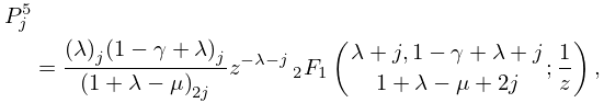
►
31.11.3_1
►
31.11.3_2
…
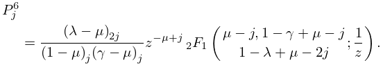
►
31.11.12
…
