Legendre%0Aelliptic%20integrals

SearchAdvancedHelp

(0.003 seconds)

21—30 of 807 matching pages

21: 14.17 Integrals

… ►

§14.17(ii) Barnes’ Integral

… ►

§14.17(iii) Orthogonality Properties

… ►

§14.17(iv) Definite Integrals of Products

… ►

§14.17(v) Laplace Transforms

… ►

§14.17(vi) Mellin Transforms

…

22: 14.26 Uniform Asymptotic Expansions

§14.26 Uniform Asymptotic Expansions

►The uniform asymptotic approximations given in §14.15 for $P_{\nu }^{-\mu }\left(x\right)$ and ${𝑸}_{\nu }^{\mu }\left(x\right)$ for are extended to domains in the complex plane in the following references: §§14.15(i) and 14.15(ii), Dunster (2003b); §14.15(iii), Olver (1997b, Chapter 12); §14.15(iv), Boyd and Dunster (1986). … ►See also Frenzen (1990), Gil et al. (2000), Shivakumar and Wong (1988), Ursell (1984), and Wong (1989) for uniform asymptotic approximations obtained from integral representations.

23: 14.31 Other Applications

… ►The conical functions ${𝖯}_{-\frac{1}{2}+\mathrm{i}\tau }^m\left(x\right)$ appear in boundary-value problems for the Laplace equation in toroidal coordinates (§14.19(i)) for regions bounded by cones, by two intersecting spheres, or by one or two confocal hyperboloids of revolution (Kölbig (1981)). … ►

§14.31(iii) Miscellaneous

►Many additional physical applications of Legendre polynomials and associated Legendre functions include solution of the Helmholtz equation, as well as the Laplace equation, in spherical coordinates (Temme (1996b)), quantum mechanics (Edmonds (1974)), and high-frequency scattering by a sphere (Nussenzveig (1965)). … ►Legendre functions $P_{\nu }\left(x\right)$ of complex degree $\nu$ appear in the application of complex angular momentum techniques to atomic and molecular scattering (Connor and Mackay (1979)).

24: 14.10 Recurrence Relations and Derivatives

§14.10 Recurrence Relations and Derivatives

… ► ${𝖰}_{\nu }^{\mu }\left(x\right)$ also satisfies (14.10.1)–(14.10.5). ►

14.10.6 $$P_{\nu }^{\mu +2}\left(x\right)+2(\mu +1)x{\left(x^2-1\right)}^{-1/2}{P}_{\nu }^{\mu +1}\left(x\right)-(\nu -\mu )(\nu +\mu +1)P_{\nu }^{\mu }\left(x\right)=0,$$

ⓘ

Symbols:

$P_{\nu }^{\mu }\left(z\right)$: associated Legendre function of the first kind, $x$: real variable, $\mu$: general order and $\nu$: general degree

Referenced by:

§14.10, §14.14

Permalink:

http://dlmf.nist.gov/14.10.E6

Encodings:

pMML, png, TeX

See also:

Annotations for §14.10 and Ch.14

… ► $Q_{\nu }^{\mu }\left(x\right)$ also satisfies (14.10.6) and (14.10.7). In addition, $P_{\nu }^{\mu }\left(x\right)$ and $Q_{\nu }^{\mu }\left(x\right)$ satisfy (14.10.3)–(14.10.5).

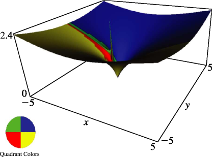
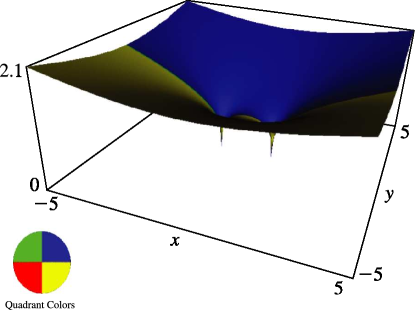
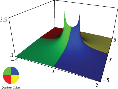
25: 14.22 Graphics

§14.22 Graphics

… ►

►

►

Figure 14.22.1: $P_{1/2}^0\left(x+\mathrm{i}y\right)$, $-5\le x\le 5$, $-5\le y\le 5$. … Magnify 3D Help

►

►

►

Figure 14.22.2: $P_{1/2}^{-1/2}\left(x+\mathrm{i}y\right)$, $-5\le x\le 5$, $-5\le y\le 5$. … Magnify 3D Help

… ►

►

►

Figure 14.22.4: ${𝑸}_0^0\left(x+\mathrm{i}y\right)$, $-5\le x\le 5$, $-5\le y\le 5$. … Magnify 3D Help

26: 14.28 Sums

§14.28 Sums

►

§14.28(i) Addition Theorem

►When $\mathrm{\Re }{z}_1>0$, $\mathrm{\Re }{z}_2>0$, , and , …where the branches of the square roots have their principal values when $z_1,z_2\in (1,\mathrm{\infty })$ and are continuous when $z_1,z_2\in ℂ\setminus (0,1]$. … ►

§14.28(ii) Heine’s Formula

…

27: 14.12 Integral Representations

§14.12 Integral Representations

… ►

§14.12(ii)

… ►

Neumann’s Integral

… ►

Heine’s Integral

… ►For further integral representations see Erdélyi et al. (1953a, pp. 158–159) and Magnus et al. (1966, pp. 184–190), and for contour integrals and other representations see §14.25.

28: 19.35 Other Applications

… ►

§19.35(i) Mathematical

►Generalizations of elliptic integrals appear in analysis of modular theorems of Ramanujan (Anderson et al. (2000)); analysis of Selberg integrals (Van Diejen and Spiridonov (2001)); use of Legendre’s relation (19.7.1) to compute $\pi$ to high precision (Borwein and Borwein (1987, p. 26)). ►

§19.35(ii) Physical

… ►

29: 14.27 Zeros

§14.27 Zeros

► $P_{\nu }^{\mu }\left(x\pm \mathrm{i}0\right)$ (either side of the cut) has exactly one zero in the interval $(-\mathrm{\infty },-1)$ if either of the following sets of conditions holds: … ►

$\mu ,\nu \in \mathbb{Z}$, , and $\nu$ is odd.

►For all other values of the parameters $P_{\nu }^{\mu }\left(x\pm \mathrm{i}0\right)$ has no zeros in the interval $(-\mathrm{\infty },-1)$. ►For complex zeros of $P_{\nu }^{\mu }\left(z\right)$ see Hobson (1931, §§233, 234, and 238).

30: 19.38 Approximations

§19.38 Approximations

►Minimax polynomial approximations (§3.11(i)) for $K\left(k\right)$ and $E\left(k\right)$ in terms of $m=k^2$ with can be found in Abramowitz and Stegun (1964, §17.3) with maximum absolute errors ranging from 4×10⁻⁵ to 2×10⁻⁸. Approximations of the same type for $K\left(k\right)$ and $E\left(k\right)$ for are given in Cody (1965a) with maximum absolute errors ranging from 4×10⁻⁵ to 4×10⁻¹⁸. … ►Approximations for Legendre’s complete or incomplete integrals of all three kinds, derived by Padé approximation of the square root in the integrand, are given in Luke (1968, 1970). …