Cash App Wallet Phone%E2%98%8E%EF%B8%8F%2B1%28888%E2%80%92481%E2%80%924477%29%E2%98%8E%EF%B8%8F %22Number%22
(0.020 seconds)
11—20 of 859 matching pages
11: 29.17 Other Solutions
…
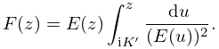
►If (29.2.1) admits a Lamé polynomial solution , then a second linearly independent solution is given by
►
29.17.1
…
►They are algebraic functions of , , and , and have primitive period .
…
►Lamé–Wangerin functions are solutions of (29.2.1) with the property that is bounded on the line segment from to .
…
12: 3.1 Arithmetics and Error Measures
…
►with and all allowable choices of , , , and .
…
►Let with and .
For given values of , , and , the format width in bits
of a computer word is the total number of bits: the sign (one bit), the significant bits ( bits), and the bits allocated to the exponent (the remaining bits).
The integers , , and are characteristics of the machine.
…
►In the case of the normalized binary interchange formats, the representation of data for binary32 (previously single precision) (, , , ), binary64 (previously double precision) (, , , ) and binary128 (previously quad precision) (, , , ) are as in Figure 3.1.1.
…
13: 6.20 Approximations
…
►
•
►
•
…
►
•
…
►
•
…
►
•
…
Cody and Thacher (1968) provides minimax rational approximations for , with accuracies up to 20S.
Clenshaw (1962) gives Chebyshev coefficients for for and for (20D).
Luke (1969b, pp. 321–322) covers and for (the Chebyshev coefficients are given to 20D); for (20D), and for (15D). Coefficients for the sine and cosine integrals are given on pp. 325–327.
Luke (1969b, pp. 402, 410, and 415–421) gives main diagonal Padé approximations for , , (valid near the origin), and (valid for large ); approximate errors are given for a selection of -values.
14: Bibliography O
…
►
Summing one- and two-dimensional series related to the Euler series.
J. Comput. Appl. Math. 98 (2), pp. 245–271.
…
►
Uniform asymptotic expansions for hypergeometric functions with large parameters. III.
Analysis and Applications (Singapore) 8 (2), pp. 199–210.
…
►
Connection formulas for second-order differential equations with multiple turning points.
SIAM J. Math. Anal. 8 (1), pp. 127–154.
►
Connection formulas for second-order differential equations having an arbitrary number of turning points of arbitrary multiplicities.
SIAM J. Math. Anal. 8 (4), pp. 673–700.
…
►
Numerical evaluation of the dilogarithm of complex argument.
Celestial Mech. Dynam. Astronom. 62 (1), pp. 93–98.
…
15: 34.5 Basic Properties: Symbol
…
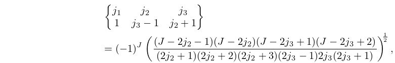
►If any lower argument in a symbol is , , or , then the symbol has a simple algebraic form.
…
►
34.5.6
…
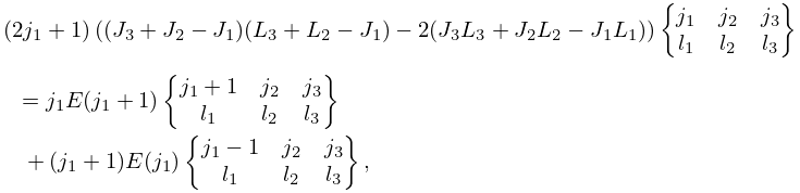
►
34.5.11
…
►
34.5.13
►For further recursion relations see Varshalovich et al. (1988, §9.6) and Edmonds (1974, pp. 98–99).
…
16: 24.9 Inequalities
§24.9 Inequalities
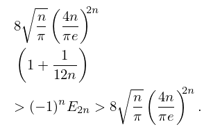
►Except where otherwise noted, the inequalities in this section hold for . … ►(24.9.3)–(24.9.5) hold for . … ►(24.9.6)–(24.9.7) hold for . … ►
24.9.7
…
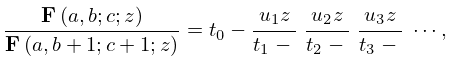
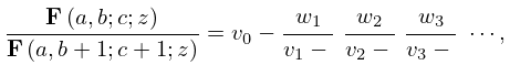
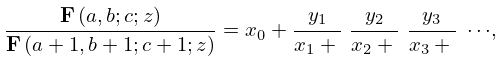
17: 15.7 Continued Fractions
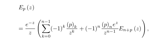
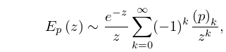
18: 8.20 Asymptotic Expansions of
§8.20 Asymptotic Expansions of
… ►
8.20.1
.
…
►
8.20.2
,
…
►For an exponentially-improved asymptotic expansion of see §2.11(iii).
…
►
19: 24.20 Tables
§24.20 Tables
►Abramowitz and Stegun (1964, Chapter 23) includes exact values of , , ; , , , , 20D; , , 18D. ►Wagstaff (1978) gives complete prime factorizations of and for and , respectively. In Wagstaff (2002) these results are extended to and , respectively, with further complete and partial factorizations listed up to and , respectively. …20: 19.36 Methods of Computation
…
►where the elementary symmetric functions are defined by (19.19.4).
If (19.36.1) is used instead of its first five terms, then the factor in Carlson (1995, (2.2)) is changed to .
…
►Thompson (1997, pp. 499, 504) uses descending Landen transformations for both and .
…
►If , then the method fails, but the function can be expressed by (19.6.13) in terms of , for which Neuman (1969b) uses ascending Landen transformations.
…
►Lee (1990) compares the use of theta functions for computation of , , and , , with four other methods.
…
