Bernoulli
(0.001 seconds)
31—40 of 66 matching pages
31: 17.3 -Elementary and -Special Functions
…
►
§17.3(iii) Bernoulli Polynomials; Euler and Stirling Numbers
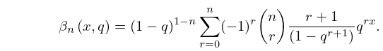
►-Bernoulli Polynomials
►
17.3.7
…
►The are, in fact, rational functions of , and not necessarily polynomials.
…
32: 5.15 Polygamma Functions
33: 2.10 Sums and Sequences
…
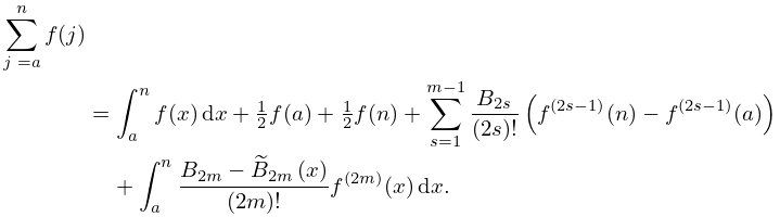
►As in §24.2, let and denote the th Bernoulli number and polynomial, respectively, and the th Bernoulli periodic function .
…
►
2.10.1
…
►
2.10.4
…
►
2.10.5
►From §24.12(i), (24.2.2), and (24.4.27), is of constant sign .
…
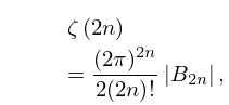
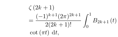
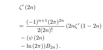
34: 25.6 Integer Arguments
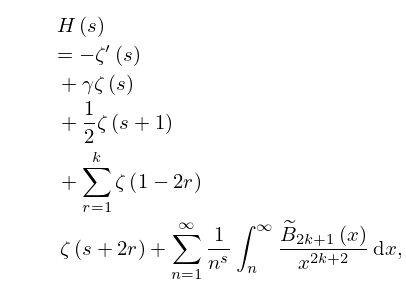
35: 25.16 Mathematical Applications
…
►
25.16.6
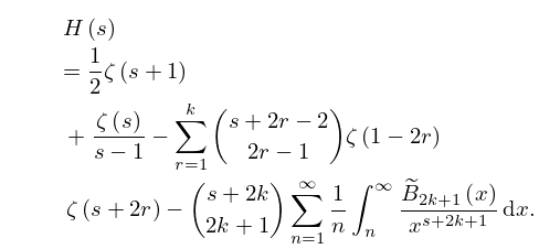
►
25.16.7
…
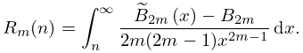
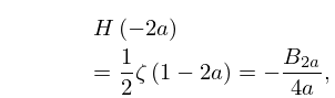
►
25.16.10
.
►
has a simple pole with residue () at each odd negative integer , .
…
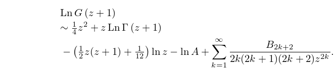
36: 5.17 Barnes’ -Function (Double Gamma Function)
37: Bibliography D
…
►
Sur les zéros réels des polynômes de Bernoulli.
Ann. Inst. Fourier (Grenoble) 41 (2), pp. 267–309 (French).
…
►
Asymptotic behaviour of Bernoulli, Euler, and generalized Bernoulli polynomials.
J. Approx. Theory 49 (4), pp. 321–330.
…
►
Zeros of Bernoulli, generalized Bernoulli and Euler polynomials.
Mem. Amer. Math. Soc. 73 (386), pp. iv+94.
►
Sums of products of Bernoulli numbers.
J. Number Theory 60 (1), pp. 23–41.
►
Bernoulli Numbers and Confluent Hypergeometric Functions.
In Number Theory for the Millennium, I (Urbana, IL, 2000),
pp. 343–363.
…
38: 19.30 Lengths of Plane Curves
39: Bibliography T
…
►
New congruences for the Bernoulli numbers.
Math. Comp. 48 (177), pp. 341–350.
…
►
Bernoulli polynomials old and new: Generalizations and asymptotics.
CWI Quarterly 8 (1), pp. 47–66.
…
►
Explicit formulas for the Bernoulli and Euler polynomials and numbers.
Abh. Math. Sem. Univ. Hamburg 61, pp. 175–180.
…
►
On the theory of the Bernoulli polynomials and numbers.
J. Math. Anal. Appl. 104 (2), pp. 309–350.
…
40: Bibliography H
…
►
An Euler-Maclaurin-type formula involving conjugate Bernoulli polynomials and an application to
.
Commun. Appl. Anal. 1 (1), pp. 15–32.
…
►
An explicit formula for Bernoulli numbers.
Rep. Fac. Sci. Technol. Meijo Univ. 29, pp. 1–6.
►
On congruences involving Bernoulli numbers and irregular primes. II.
Rep. Fac. Sci. Technol. Meijo Univ. 31, pp. 1–8.
…
►
Explicit formulas for degenerate Bernoulli numbers.
Discrete Math. 162 (1-3), pp. 175–185.
…
►
Bernoulli numbers and polynomials via residues.
J. Number Theory 76 (2), pp. 178–193.
…
