.%E8%81%94%E9%80%9A%E7%9B%92%E5%AD%90%E6%80%8E%E4%B9%88%E7%9C%8B%E4%B8%96%E7%95%8C%E6%9D%AF_%E3%80%8Ewn4.com_%E3%80%8F%E4%B8%96%E7%95%8C%E6%9D%AF%E8%B5%8C%E7%90%83%E5%B9%B3%E4%BA%86%E6%80%8E%E4%B9%88%E7%AE%97_w6n2c9o_2022%E5%B9%B411%E6%9C%8829%E6%97%A55%E6%97%B631%E5%88%8638%E7%A7%92_m2c8qeq0s
(0.026 seconds)
21—30 of 670 matching pages
21: 26.14 Permutations: Order Notation
…
►As an example, is an element of The inversion number is the number of pairs of elements for which the larger element precedes the smaller:
…
►The permutation has two descents: and .
…For example, .
…
►In this subsection is again the Stirling number of the second kind (§26.8), and is the th Bernoulli number (§24.2(i)).
…
►
26.14.11
.
…
22: 1.3 Determinants, Linear Operators, and Spectral Expansions
…
►Square matices can be seen as linear operators because for all and , the space of all -dimensional vectors.
…
►The adjoint of a matrix is the matrix such that for all .
In the case of a real matrix and in the complex case .
►Real symmetric () and Hermitian () matrices are self-adjoint operators on .
…
►For self-adjoint and , if , see (1.2.66), simultaneous eigenvectors of and always exist.
…
23: 25.16 Mathematical Applications
…
►
25.16.2
,
…
►where is given by (25.11.33).
…
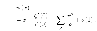
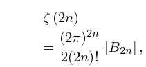
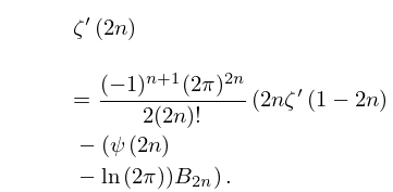
►
has a simple pole with residue () at each odd negative integer , .
…
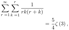
►
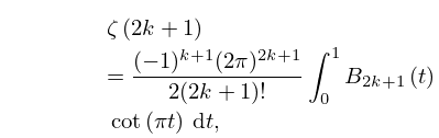
25.16.14
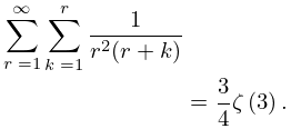
►
25.16.15
…
24: 11.11 Asymptotic Expansions of Anger–Weber Functions
…
►Let , and for ,
…
►
.
…
►When is real and positive, all of (11.11.10)–(11.11.17) can be regarded as special cases of two asymptotic expansions given in Olver (1997b, pp. 352–360) for as , one being uniform for , and the other being uniform for .
(Note that Olver’s definition of omits the factor in (11.10.4).)
…
►Lastly, corresponding asymptotic approximations and expansions for and , with or , follow from (11.10.15) and (11.10.16) and the corresponding asymptotic expansions for the Bessel functions and ; see §10.19(ii).
…
25: Bibliography M
…
►
Formulas and Theorems for the Special Functions of Mathematical Physics.
3rd edition, Springer-Verlag, New York-Berlin.
…
►
On the Representation of Meijer’s -Function in the Vicinity of Singular Unity.
In Complex Analysis and Applications ’81 (Varna, 1981),
pp. 383–398.
…
►
On the roots of the Bessel and certain related functions.
Ann. of Math. 9 (1-6), pp. 23–30.
…
►
Orthogonale Polynomsysteme mit einer besonderen Gestalt der erzeugenden Funktion.
J. Lond. Math. Soc. 9, pp. 6–13 (German).
…
►
The -analogue of the Laguerre polynomials.
J. Math. Anal. Appl. 81 (1), pp. 20–47.
…
26: Bibliography B
…
►
Numerical evaluation of the zero-order Hankel transform using Filon quadrature philosophy.
Appl. Math. Lett. 9 (5), pp. 21–26.
…
►
Avoided crossings of the quartic oscillator.
J. Phys. A 30 (9), pp. 3057–3067.
…
►
Methods of calculation of radial wave functions and new tables of Coulomb functions.
Physical Rev. (2) 80, pp. 553–560.
…
►
Algorithm 524: MP, A Fortran multiple-precision arithmetic package [A1].
ACM Trans. Math. Software 4 (1), pp. 71–81.
…
►
The determination of phases and amplitudes of wave functions.
Proc. Phys. Soc. 81 (3), pp. 442–452.
…
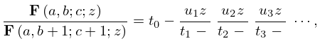
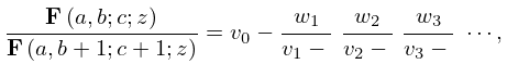
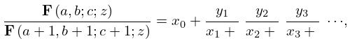
27: 15.7 Continued Fractions
28: 25.6 Integer Arguments
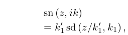
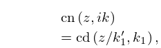
29: 22.17 Moduli Outside the Interval [0,1]
30: 3.5 Quadrature
…
►If , then the remainder in (3.5.2) can be expanded in the form
…
►For the Bernoulli numbers see §24.2(i).
…
►About function evaluations are needed.
…
►with weight function
, is one for which whenever is a polynomial of degree .
…
►For further information, see Mason and Handscomb (2003, Chapter 8), Davis and Rabinowitz (1984, pp. 74–92), and Clenshaw and Curtis (1960).
…
