%E6%A3%8B%E7%89%8C%E6%B8%B8%E6%88%8F%E4%B8%8B%E8%BD%BD,%E7%8E%B0%E9%87%91%E6%A3%8B%E7%89%8C%E5%B9%B3%E5%8F%B0,%E7%9C%9F%E4%BA%BA%E6%A3%8B%E7%89%8C%E5%AE%98%E7%BD%91,%E3%80%90%E6%A3%8B%E7%89%8C%E6%B8%B8%E6%88%8F%E7%BD%91%E5%9D%80%E2%88%B6789yule.com%E3%80%91%E7%9C%9F%E4%BA%BA%E7%9C%9F%E9%92%B1%E6%A3%8B%E7%89%8C%E6%B8%B8%E6%88%8F,%E7%BD%91%E4%B8%8A%E6%A3%8B%E7%89%8C%E8%AE%BA%E5%9D%9B,%E7%BD%91%E7%BB%9C%E5%8D%9A%E5%BD%A9%E8%AE%BA%E5%9D%9B,%E6%A3%8B%E7%89%8C%E6%B8%B8%E6%88%8F%E8%B5%8C%E5%8D%9A%E7%BD%91%E7%AB%99,%E3%80%90%E6%A3%8B%E7%89%8C%E6%B8%B8%E6%88%8F%E7%BD%91%E7%AB%99%E2%88%B6789yule.com%E3%80%91%E7%BD%91%E5%9D%80ZDg0nAkCfB0BknED

SearchAdvancedHelp

(0.070 seconds)

21—30 of 616 matching pages

21: 14.33 Tables

… ►

Abramowitz and Stegun (1964, Chapter 8) tabulates ${𝖯}_n\left(x\right)$ for $n=0(1)3,9,10$, $x=0(.01)1$, 5–8D; ${𝖯}_n^{\prime }\left(x\right)$ for $n=1(1)4,9,10$, $x=0(.01)1$, 5–7D; ${𝖰}_n\left(x\right)$ and ${𝖰}_n^{\prime }\left(x\right)$ for $n=0(1)3,9,10$, $x=0(.01)1$, 6–8D; $P_n\left(x\right)$ and $P_n^{\prime }\left(x\right)$ for $n=0(1)5,9,10$, $x=1(.2)10$, 6S; $Q_n\left(x\right)$ and $Q_n^{\prime }\left(x\right)$ for $n=0(1)3,9,10$, $x=1(.2)10$, 6S. (Here primes denote derivatives with respect to $x$.)

►

Zhang and Jin (1996, Chapter 4) tabulates ${𝖯}_n\left(x\right)$ for $n=2(1)5,10$, $x=0(.1)1$, 7D; ${𝖯}_n\left(\cos \theta \right)$ for $n=1(1)4,10$, $\theta =0(5^{\circ }){90}^{\circ }$, 8D; ${𝖰}_n\left(x\right)$ for $n=0(1)2,10$, $x=0(.1)0.9$, 8S; ${𝖰}_n\left(\cos \theta \right)$ for $n=0(1)3,10$, $\theta =0(5^{\circ }){90}^{\circ }$, 8D; ${𝖯}_n^m\left(x\right)$ for $m=1(1)4$, $n-m=0(1)2$, $n=10$, $x=0,0.5$, 8S; ${𝖰}_n^m\left(x\right)$ for $m=1(1)4$, $n=0(1)2,10$, 8S; ${𝖯}_{\nu }^m\left(\cos \theta \right)$ for $m=0(1)3$, $\nu =0(.25)5$, $\theta =0({15}^{\circ }){90}^{\circ }$, 5D; $P_n\left(x\right)$ for $n=2(1)5,10$, $x=1(1)10$, 7S; $Q_n\left(x\right)$ for $n=0(1)2,10$, $x=2(1)10$, 8S. Corresponding values of the derivative of each function are also included, as are 6D values of the first 5 $\nu$-zeros of ${𝖯}_{\nu }^m\left(\cos \theta \right)$ and of its derivative for $m=0(1)4$, $\theta ={10}^{\circ },{30}^{\circ },{150}^{\circ }$.

►

Belousov (1962) tabulates ${𝖯}_n^m\left(\cos \theta \right)$ (normalized) for $m=0(1)36$, $n-m=0(1)56$, $\theta =0({2.5}^{\circ }){90}^{\circ }$, 6D.

…

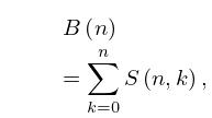
22: 26.7 Set Partitions: Bell Numbers

… ► $B\left(n\right)$ is the number of partitions of $\{1,2,\mathrm{\dots },n\}$. … ►

26.7.1 $$B\left(0\right)=1,$$

ⓘ

Symbols:

$B\left(n\right)$: Bell number

Permalink:

http://dlmf.nist.gov/26.7.E1

Encodings:

pMML, png, TeX

See also:

Annotations for §26.7(i), §26.7 and Ch.26

►

26.7.2 $$B\left(n\right)=\sum _{k=0}^{n}S(n,k),$$

ⓘ

Symbols:

$B\left(n\right)$: Bell number, $S(n,k)$: Stirling number of the second kind, $k$: nonnegative integer and $n$: nonnegative integer

Permalink:

http://dlmf.nist.gov/26.7.E2

Encodings:

pMML, png, TeX

See also:

Annotations for §26.7(i), §26.7 and Ch.26

… ►

26.7.6 $$B\left(n+1\right)=\sum _{k=0}^n\left(\genfrac{}{}{0.0pt}{}{n}{k}\right)B\left(k\right).$$

ⓘ

Symbols:

$B\left(n\right)$: Bell number, $\left(\genfrac{}{}{0.0pt}{}{m}{n}\right)$: binomial coefficient, $k$: nonnegative integer and $n$: nonnegative integer

Referenced by:

Erratum (V1.0.1) for Equation (26.7.6)

Permalink:

http://dlmf.nist.gov/26.7.E6

Encodings:

pMML, png, TeX

Errata (effective with 1.0.1):

Originally appeared with $B\left(n\right)$ in the summation, instead of $B\left(k\right)$:

$$B\left(n+1\right)=\sum _{k=0}^n\left(\genfrac{}{}{0.0pt}{}{n}{k}\right)B\left(n\right)$$

Reported 2010-11-07 by Layne Watson

See also:

Annotations for §26.7(iii), §26.7 and Ch.26

… ►For higher approximations to $B\left(n\right)$ as $n\to \mathrm{\infty }$ see de Bruijn (1961, pp. 104–108).

23: 18.8 Differential Equations

… ►

Table 18.8.1: Classical OP’s: differential equations $A(x)f^{\prime \prime }(x)+B(x)f^{\prime }(x)+C(x)f(x)+{\lambda }_{n}f(x)=0$.

► ►►►►►

#	$f(x)$	$A(x)$	$B(x)$	$C(x)$	${\lambda }_n$
…
4	$C_n^{(\lambda )}\left(x\right)$	$1-x^2$	$-(2\lambda +1)x$	$0$	$n(n+2\lambda )$
…
8	$L_n^{(\alpha )}\left(x\right)$	$x$	$\alpha +1-x$	$0$	$n$
9	${\mathrm{e}}^{-\frac{1}{2}{x}^2}{x}^{\alpha +\frac{1}{2}}{L}_n^{(\alpha )}\left(x^2\right)$	$1$	$0$	$-x^2+(\frac{1}{4}-{\alpha }^2)x^{-2}$	$4n+2\alpha +2$
…

►

…

24: Bibliography D

… ►

The principal frequencies of vibrating systems with elliptic boundaries. Quart. J. Mech. Appl. Math. 8 (3), pp. 361–372.

ⓘ

External Links:

Document, MathReview (M. A. Hyman), ZentralBlatt

Referenced by:

3rd item.

Encodings:

BibTeX

… ►

Handbuch der Laplace-Transformation. Bd. II. Anwendungen der Laplace-Transformation. 1. Abteilung. Birkhäuser Verlag, Basel und Stuttgart (German).

ⓘ

External Links:

MathReview (I. I. Hirschman), ZentralBlatt

Referenced by:

§2.5(i).

Encodings:

BibTeX

… ►

Inequalities for extreme zeros of some classical orthogonal and $q$-orthogonal polynomials. Math. Model. Nat. Phenom. 8 (1), pp. 48–59.

ⓘ

External Links:

ISSN 0973-5348, Document, FullText, MathReview (Ana Foulquié Moreno), ZentralBlatt

Referenced by:

§18.16(ii), §18.16(iv), §18.16(ii), §18.16(iv), §18.27(iv), §18.27(iv), §18.27(v), §18.27(v).

Encodings:

BibTeX

… ►

Lamé instantons. J. High Energy Phys. 2000 (1), pp. Paper 19, 8.

ⓘ

Notes:

(electronic only, article id. JHEP01(2000)019, 8 pp.).

External Links:

ISSN 1029-8479, Document, MathReview, ZentralBlatt

Referenced by:

§22.11.

Encodings:

BibTeX

… ►

Product formulas and Nicholson-type integrals for Jacobi functions. I. Summary of results. SIAM J. Math. Anal. 9 (1), pp. 76–86.

ⓘ

External Links:

Document, MathReview (R. C. Varma), ZentralBlatt

Referenced by:

§18.17(iii).

Encodings:

BibTeX

…

25: 3.5 Quadrature

… ►If in addition $f$ is periodic, $f\in C^k(ℝ)$, and the integral is taken over a period, then … ►If $f\in C^{2m+2}[a,b]$, then the remainder $E_n(f)$ in (3.5.2) can be expanded in the form … ►For the Bernoulli numbers $B_m$ see §24.2(i). … ►For further information, see Mason and Handscomb (2003, Chapter 8), Davis and Rabinowitz (1984, pp. 74–92), and Clenshaw and Curtis (1960). … ►For $C^{\mathrm{\infty }}$ functions Gauss quadrature can be very efficient. …

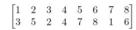
26: 26.13 Permutations: Cycle Notation

… ►

26.13.2

ⓘ

Referenced by:

§26.13, §26.13, §26.13

Permalink:

http://dlmf.nist.gov/26.13.E2

Encodings:

pMML, png, TeX

See also:

Annotations for §26.13 and Ch.26

►is $\left(1,3,2,5,7\right)\left(4\right)\left(6,8\right)$ in cycle notation. …In consequence, (26.13.2) can also be written as $\left(1,3,2,5,7\right)\left(6,8\right)$. … ►For the example (26.13.2), this decomposition is given by $\left(1,3,2,5,7\right)\left(6,8\right)=\left(1,3\right)\left(2,3\right)\left(2,5\right)\left(5,7\right)\left(6,8\right).$ … ►Again, for the example (26.13.2) a minimal decomposition into adjacent transpositions is given by $\left(1,3,2,5,7\right)\left(6,8\right)=\left(2,3\right)\left(1,2\right)\left(4,5\right)\left(3,4\right)\left(2,3\right)\left(3,4\right)\left(4,5\right)\left(6,7\right)\left(5,6\right)\left(7,8\right)\left(6,7\right)$: $inv(\left(1,3,2,5,7\right)\left(6,8\right))=11$.

27: 12.14 The Function $W(a,x)$

… ►For the modulus functions $\tilde{F}(a,x)$ and $\tilde{G}(a,x)$ see §12.14(x). … ►Other expansions, involving $\cos \left(\frac{1}{4}{x}^2\right)$ and $\sin \left(\frac{1}{4}{x}^2\right)$, can be obtained from (12.4.3) to (12.4.6) by replacing $a$ by $-\mathrm{i}a$ and $z$ by $x{\mathrm{e}}^{\pi \mathrm{i}/4}$; see Miller (1955, p. 80), and also (12.14.15) and (12.14.16). … ►uniformly for $t\in [-1+\delta ,\mathrm{\infty })$, with $\zeta$, $\varphi (\zeta )$, $A_s(\zeta )$, and $B_s(\zeta )$ as in §12.10(vii). … ► $\tilde{F}$ or $\tilde{G}$ is the modulus and $\tilde{\theta }$ or $\tilde{\psi }$ is the corresponding phase. … ►For properties of the modulus and phase functions, including differential equations and asymptotic expansions for large $x$, see Miller (1955, pp. 87–88). …

28: 2.10 Sums and Sequences

… ►For further information on $C$ see §5.17. … ►For extensions to $\alpha \le 0$, higher terms, and other examples, see Olver (1997b, Chapter 8). … ►For generalizations and other examples see Olver (1997b, Chapter 8), Ford (1960), and Berndt and Evans (1984). … ►For examples see Olver (1997b, Chapters 8, 9). … ►For other examples and extensions see Olver (1997b, Chapter 8), Olver (1970), Wong (1989, Chapter 2), and Wong and Wyman (1974). …

29: 1.11 Zeros of Polynomials

… ►Set $z=w-\frac{1}{3}a$ to reduce $f(z)=z^3+a{z}^2+bz+c$ to $g(w)=w^3+pw+q$, with $p=(3b-a^2)/3$, $q=(2a^3-9ab+27c)/27$. … ► $f(z)=z^3-6z^2+6z-2$, $g(w)=w^3-6w-6$, $A=3\sqrt[3]{4}$, $B=3\sqrt[3]{2}$. … ►Resolvent cubic is $z^3+12z^2+20z+9=0$ with roots ${\theta }_1=-1$, ${\theta }_2=-\frac{1}{2}(11+\sqrt{85})$, ${\theta }_3=-\frac{1}{2}(11-\sqrt{85})$, and $\sqrt{-{\theta }_1}=1$, $\sqrt{-{\theta }_2}=\frac{1}{2}(\sqrt{17}+\sqrt{5})$, $\sqrt{-{\theta }_3}=\frac{1}{2}(\sqrt{17}-\sqrt{5})$. … ►Let … ►Then $f(z)$, with $a_n\ne 0$, is stable iff $a_0\ne 0$; $D_{2k}>0$, $k=1,\mathrm{\dots },\lfloor \frac{1}{2}n\rfloor$; $\mathrm{sign}{D}_{2k+1}=\mathrm{sign}{a}_0$, $k=0,1,\mathrm{\dots },\lfloor \frac{1}{2}n-\frac{1}{2}\rfloor$.

30: Bibliography L

… ►

On the maxima and minima of Bernoulli polynomials. Amer. Math. Monthly 47 (8), pp. 533–538.

ⓘ

External Links:

FullText, MathReview (W. E. Milne), ZentralBlatt

Referenced by:

§24.12(i), §24.9.

Encodings:

BibTeX

… ►

A partition function connected with the modulus five. Duke Math. J. 8 (4), pp. 631–655.

ⓘ

External Links:

Document, MathReview (R. D. James), ZentralBlatt

Referenced by:

§17.18.

Encodings:

BibTeX

… ►

On the theory of diffraction by an aperture in an infinite plane screen. I. Phys. Rev. 74 (8), pp. 958–974.

ⓘ

External Links:

Document, MathReview (C. J. Bouwkamp), ZentralBlatt

Referenced by:

§11.12.

Encodings:

BibTeX

… ►

Monotonicity and convexity properties of zeros of Bessel functions. SIAM J. Math. Anal. 8 (1), pp. 171–178.

ⓘ

External Links:

ISSN 1095-7154, Document, MathReview (T. Erber), ZentralBlatt

Referenced by:

§10.21(iv).

Encodings:

BibTeX

… ►

Solutions of the fifth Painlevé equation. Differ. Uravn. 4 (8), pp. 1413–1420 (Russian).

ⓘ

Notes:

In Russian. English translation: Differential Equations 4(8), pp. 732–735

External Links:

MathReview (C. E. Langenhop), ZentralBlatt

Referenced by:

§32.10(v), §32.8(v).

Encodings:

BibTeX

…