%E6%A2%AD%E5%93%88%E6%B8%B8%E6%88%8F%E5%A4%A7%E5%8E%85,%E7%BD%91%E4%B8%8A%E6%A2%AD%E5%93%88%E6%B8%B8%E6%88%8F%E8%A7%84%E5%88%99,%E3%80%90%E5%A4%8D%E5%88%B6%E6%89%93%E5%BC%80%E7%BD%91%E5%9D%80%EF%BC%9A33kk55.com%E3%80%91%E6%AD%A3%E8%A7%84%E5%8D%9A%E5%BD%A9%E5%B9%B3%E5%8F%B0,%E5%9C%A8%E7%BA%BF%E8%B5%8C%E5%8D%9A%E5%B9%B3%E5%8F%B0,%E6%A2%AD%E5%93%88%E6%B8%B8%E6%88%8F%E7%8E%A9%E6%B3%95%E4%BB%8B%E7%BB%8D,%E7%9C%9F%E4%BA%BA%E6%A2%AD%E5%93%88%E6%B8%B8%E6%88%8F%E8%A7%84%E5%88%99,%E7%BD%91%E4%B8%8A%E7%9C%9F%E4%BA%BA%E6%A3%8B%E7%89%8C%E6%B8%B8%E6%88%8F%E5%B9%B3%E5%8F%B0,%E7%9C%9F%E4%BA%BA%E5%8D%9A%E5%BD%A9%E6%B8%B8%E6%88%8F%E5%B9%B3%E5%8F%B0%E7%BD%91%E5%9D%80YCBNyMNNVhsBhNMy

(0.075 seconds)

31—40 of 673 matching pages

31: 19.37 Tables

… ►

Functions $F\left(\phi,k\right)$ and $E\left(\phi,k\right)$

… ►(

F\left(\phi,k\right)

is presented as

\Pi\left(\phi,0,k\right)

.) … ►Tabulated for

\phi=5^{\circ}(5^{\circ})80^{\circ}(2.5^{\circ})90^{\circ}

\alpha^{2}=-1(.1)-0.1,0.1(.1)1

k^{2}=0(.05)0.9(.02)1

to 10D by Fettis and Caslin (1964) (and warns of inaccuracies in Selfridge and Maxfield (1958) and Paxton and Rollin (1959)). … ►

Functions $R_{F}\left(x^{2},1,y^{2}\right)$ and $R_{G}\left(x^{2},1,y^{2}\right)$

… ►

Function $R_{F}\left(a^{2},b^{2},c^{2}\right)$ with $abc=1$

…

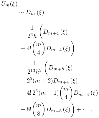
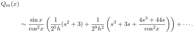
32: 28.8 Asymptotic Expansions for Large $q$

… ►

28.8.1

\rselection{a_{m}\left(h^{2}\right)\\ b_{m+1}\left(h^{2}\right)}\sim-2h^{2}+2sh-\frac{1}{8}(s^{2}+1)-\frac{1}{2^{7}h% }(s^{3}+3s)-\frac{1}{2^{12}h^{2}}(5s^{4}+34s^{2}+9)-\frac{1}{2^{17}h^{3}}(33s^% {5}+410s^{3}+405s)-\frac{1}{2^{20}h^{4}}(63s^{6}+1260s^{4}+2943s^{2}+486)-% \frac{1}{2^{25}h^{5}}(527s^{7}+15617s^{5}+69001s^{3}+41607s)+\cdots.

ⓘ

Symbols:: $a_{\NVar{n}}\left(\NVar{q}\right)$ : eigenvalues of Mathieu equation, $b_{\NVar{n}}\left(\NVar{q}\right)$ : eigenvalues of Mathieu equation, $\sim$ : Poincaré asymptotic expansion, $m$ : integer and $h$ : parameter
A&S Ref:: 20.2.30 (in different form)
Referenced by:: §28.8(i), Erratum (V1.1.10) for Sections 28.6(i), 28.6(ii), 28.8(i), 28.8(ii)
Permalink:: http://dlmf.nist.gov/28.8.E1
Encodings:: pMML, png, TeX
See also:: Annotations for §28.8(i), §28.8 and Ch.28

… ►Also let

\xi=2\sqrt{h}\cos x

and

D_{m}\left(\xi\right)=e^{-\ifrac{\xi^{2}}{4}}\mathit{He}_{m}\left(\xi\right)

(§18.3). … ►

28.8.4

U_{m}(\xi)\sim D_{m}\left(\xi\right)-\frac{1}{2^{6}h}\left(D_{m+4}\left(\xi% \right)-4!\dbinom{m}{4}D_{m-4}\left(\xi\right)\right)+\frac{1}{2^{13}h^{2}}% \left(D_{m+8}\left(\xi\right)-2^{5}(m+2)D_{m+4}\left(\xi\right)+4!\,2^{5}(m-1)% \dbinom{m}{4}D_{m-4}\left(\xi\right)+8!\genfrac{(}{)}{0.0pt}{}{m}{8}D_{m-8}% \left(\xi\right)\right)+\cdots,

ⓘ

Defines:: $U_{m}(\xi)$ : function (locally)
Symbols:: $D_{\NVar{\nu}}\left(\NVar{z}\right)$ : parabolic cylinder function, $\sim$ : Poincaré asymptotic expansion, $\genfrac{(}{)}{0.0pt}{}{\NVar{m}}{\NVar{n}}$ : binomial coefficient, $!$ : factorial (as in $n!$ ), $m$ : integer, $h$ : parameter and $\xi$ : variable
A&S Ref:: 20.9.17 (in different form)
Permalink:: http://dlmf.nist.gov/28.8.E4
Encodings:: pMML, png, TeX
See also:: Annotations for §28.8(ii), §28.8 and Ch.28

… ►

28.8.6

\widehat{C}_{m}\sim\left(\frac{\pi h}{2(m!)^{2}}\right)^{\ifrac{1}{4}}\left(1+% \frac{2m+1}{8h}+\dfrac{m^{4}+2m^{3}+263m^{2}+262m+108}{2048h^{2}}+\cdots\right% )^{-\ifrac{1}{2}},

ⓘ

Defines:: $\widehat{C}_{m}$ : coefficient (locally)
Symbols:: $\sim$ : Poincaré asymptotic expansion, $\pi$ : the ratio of the circumference of a circle to its diameter, $!$ : factorial (as in $n!$ ), $m$ : integer and $h$ : parameter
A&S Ref:: 20.9.19 (in slightly different form)
Permalink:: http://dlmf.nist.gov/28.8.E6
Encodings:: pMML, png, TeX
See also:: Annotations for §28.8(ii), §28.8 and Ch.28

… ►

28.8.12

Q_{m}(x)\sim\dfrac{\sin x}{{\cos}^{2}x}\left(\dfrac{1}{2^{5}h}(s^{2}+3)+\dfrac% {1}{2^{9}h^{2}}\left(s^{3}+3s+\dfrac{4s^{3}+44s}{{\cos}^{2}x}\right)\right)+\cdots.

ⓘ

Defines:: $Q_{m}(x)$ (locally)
Symbols:: $\sim$ : Poincaré asymptotic expansion, $\cos\NVar{z}$ : cosine function, $\sin\NVar{z}$ : sine function, $m$ : integer, $h$ : parameter and $x$ : real variable
A&S Ref:: 20.9.14 (in different form)
Permalink:: http://dlmf.nist.gov/28.8.E12
Encodings:: pMML, png, TeX
See also:: Annotations for §28.8(iii), §28.8 and Ch.28

…

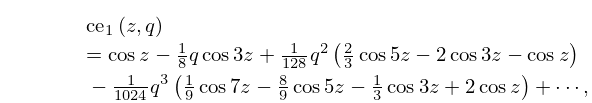
33: 28.6 Expansions for Small $q$

… ►Leading terms of the of the power series for

m=7,8,9,\dots

are: … ►Numerical values of the radii of convergence

\rho_{n}^{(j)}

of the power series (28.6.1)–(28.6.14) for

n=0,1,\dots,9

are given in Table 28.6.1. … ►where

k

is the unique root of the equation

2E\left(k\right)=K\left(k\right)

in the interval

(0,1)

, and

k^{\prime}=\sqrt{1-k^{2}}

. For

E\left(k\right)

and

K\left(k\right)

see §19.2(ii). … ►

28.6.22

\operatorname{ce}_{1}\left(z,q\right)=\cos z-\tfrac{1}{8}q\cos 3z+\tfrac{1}{12% 8}q^{2}\left(\tfrac{2}{3}\cos 5z-2\cos 3z-\cos z\right)-\tfrac{1}{1024}q^{3}% \left(\tfrac{1}{9}\cos 7z-\tfrac{8}{9}\cos 5z-\tfrac{1}{3}\cos 3z+2\cos z% \right)+\cdots,

ⓘ

Symbols:: $\operatorname{ce}_{\NVar{n}}\left(\NVar{z},\NVar{q}\right)$ : Mathieu function, $\cos\NVar{z}$ : cosine function, $q=h^{2}$ : parameter and $z$ : complex variable
Permalink:: http://dlmf.nist.gov/28.6.E22
Encodings:: pMML, png, TeX
See also:: Annotations for §28.6(ii), §28.6 and Ch.28

…

34: 10.41 Asymptotic Expansions for Large Order

… ►

U_{3}(p)=\tfrac{1}{4\;14720}\*(30375p^{3}-3\;69603p^{5}+7\;65765p^{7}-4\;25425% p^{9}),

►

V_{1}(p)=\tfrac{1}{24}(-9p+7p^{3}),

… ►The curve

E_{1}BE_{2}

in the

z

-plane is the upper boundary of the domain

\mathbf{K}

depicted in Figure 10.20.3 and rotated through an angle

-\tfrac{1}{2}\pi

. Thus

B

is the point

z=c

, where

c

is given by (10.20.18). … ►This is because

A_{k}(\zeta)

and

\zeta^{-\frac{1}{2}}B_{k}(\zeta),k=0,1,\dotsc

, do not form an asymptotic scale (§2.1(v)) as

\zeta\to+\infty

; see Olver (1997b, pp. 422–425). …

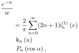
35: 10.60 Sums

… ►

10.60.3

\frac{e^{-w}}{w}=\frac{2}{\pi}\sum_{n=0}^{\infty}(2n+1){\mathsf{i}^{(1)}_{n}}% \left(v\right)\mathsf{k}_{n}\left(u\right)P_{n}\left(\cos\alpha\right),

|ve^{\pm i\alpha}|<|u|

ⓘ

Symbols:: $P_{\NVar{n}}\left(\NVar{x}\right)$ : Legendre polynomial, $\pi$ : the ratio of the circumference of a circle to its diameter, $\cos\NVar{z}$ : cosine function, $\mathrm{e}$ : base of natural logarithm, $\mathrm{i}$ : imaginary unit, ${\mathsf{i}^{(1)}_{\NVar{n}}}\left(\NVar{z}\right)$ : modified spherical Bessel function, $\mathsf{k}_{\NVar{n}}\left(\NVar{z}\right)$ : modified spherical Bessel function and $n$ : integer
A&S Ref:: 10.2.35 (with condition added)
Referenced by:: §10.60(i)
Permalink:: http://dlmf.nist.gov/10.60.E3
Encodings:: pMML, png, TeX
See also:: Annotations for §10.60(i), §10.60 and Ch.10

…

36: 18.17 Integrals

… ►For the beta function

\mathrm{B}\left(a,b\right)

see §5.12, and for the confluent hypergeometric function

{{}_{1}F_{1}}

see (16.2.1) and Chapter 13. … ►For the confluent hypergeometric function

{{}_{1}F_{1}}

see (16.2.1) and Chapter 13. … ►For the hypergeometric function

{{}_{2}F_{1}}

see §§15.1 and 15.2(i). … ►For the generalized hypergeometric function

{{}_{2}F_{2}}

see (16.2.1). … ►For further integrals, see Apelblat (1983, pp. 189–204), Erdélyi et al. (1954a, pp. 38–39, 94–95, 170–176, 259–261, 324), Erdélyi et al. (1954b, pp. 42–44, 271–294), Gradshteyn and Ryzhik (2000, pp. 788–806), Gröbner and Hofreiter (1950, pp. 23–30), Marichev (1983, pp. 216–247), Oberhettinger (1972, pp. 64–67), Oberhettinger (1974, pp. 83–92), Oberhettinger (1990, pp. 44–47 and 152–154), Oberhettinger and Badii (1973, pp. 103–112), Prudnikov et al. (1986b, pp. 420–617), Prudnikov et al. (1992a, pp. 419–476), and Prudnikov et al. (1992b, pp. 280–308).

37: 16.4 Argument Unity

… ►The function

{{}_{q+1}F_{q}}\left(\mathbf{a};\mathbf{b};z\right)

is well-poised if … ►See Raynal (1979) for a statement in terms of

\mathit{3j}

symbols (Chapter 34). … ► … ►Transformations for both balanced

{{}_{4}F_{3}}\left(1\right)

and very well-poised

{{}_{7}F_{6}}\left(1\right)

are included in Bailey (1964, pp. 56–63). A similar theory is available for very well-poised

{{}_{9}F_{8}}\left(1\right)

’s which are 2-balanced. …

38: 2.11 Remainder Terms; Stokes Phenomenon

… ►Owing to the factor

e^{-\rho}

, that is,

e^{-|z|}

in (2.11.13),

F_{n+p}\left(z\right)

is uniformly exponentially small compared with

E_{p}\left(z\right)

. … ►However, to enjoy the resurgence property (§2.7(ii)) we often seek instead expansions in terms of the

F

-functions introduced in §2.11(iii), leaving the connection of the error-function type behavior as an implicit consequence of this property of the

F

-functions. In this context the

F

-functions are called terminants, a name introduced by Dingle (1973). … ►with

m=0,1,2,\dots

, and

C_{1},C_{2}

as in (2.7.17). … ►By

n=10

we already have 8 correct decimals. …

39: 26.11 Integer Partitions: Compositions

… ►

c\left(n\right)

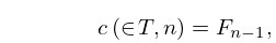
denotes the number of compositions of

n

, and

c_{m}\left(n\right)

is the number of compositions into exactly

m

parts.

c\left(\in\!T,n\right)

is the number of compositions of

n

with no 1’s, where again

T=\{2,3,4,\ldots\}

. … ►The Fibonacci numbers are determined recursively by ►

F_{0}=0

… ►

26.11.6

c\left(\in\!T,n\right)=F_{n-1},

n\geq 1

ⓘ

Symbols:: $\in$ : element of, $c\left(\NVar{\mathrm{condition}},\NVar{n}\right)$ : restricted number of compositions of $n$ , $n$ : nonnegative integer, $T$ : set and $F_{n}$ : Fibonacci numbers
Permalink:: http://dlmf.nist.gov/26.11.E6
Encodings:: pMML, png, TeX
See also:: Annotations for §26.11 and Ch.26

…

40: 30.3 Eigenvalues

… ►

30.3.11

\ell_{8}=2(4m^{2}-1)^{2}A+\frac{1}{16}B+\frac{1}{8}C+\frac{1}{2}D,

ⓘ

Symbols:: $m$ : nonnegative integer, $\ell_{j}$ : coefficients, $A$ , $B$ , $C$ and $D$
Permalink:: http://dlmf.nist.gov/30.3.E11
Encodings:: pMML, png, TeX
See also:: Annotations for §30.3(iv), §30.3 and Ch.30

►

A=\frac{(n-m-1)(n-m)(n+m-1)(n+m)}{(2n-5)^{2}(2n-3)(2n-1)^{7}(2n+1)(2n+3)^{2}}-% \frac{(n-m+1)(n-m+2)(n+m+1)(n+m+2)}{(2n-1)^{2}(2n+1)(2n+3)^{7}(2n+5)(2n+7)^{2}},

►

B=\frac{(n-m-3)(n-m-2)(n-m-1)(n-m)(n+m-3)(n+m-2)(n+m-1)(n+m)}{(2n-7)(2n-5)^{2}% (2n-3)^{3}(2n-1)^{4}(2n+1)}-\frac{(n-m+1)(n-m+2)(n-m+3)(n-m+4)(n+m+1)(n+m+2)(n% +m+3)(n+m+4)}{(2n+1)(2n+3)^{4}(2n+5)^{3}(2n+7)^{2}(2n+9)},

►

C=\frac{(n-m+1)^{2}(n-m+2)^{2}(n+m+1)^{2}(n+m+2)^{2}}{(2n+1)^{2}(2n+3)^{7}(2n+% 5)^{2}}-\frac{(n-m-1)^{2}(n-m)^{2}(n+m-1)^{2}(n+m)^{2}}{(2n-3)^{2}(2n-1)^{7}(2% n+1)^{2}},

►

D=\frac{(n-m-1)(n-m)(n-m+1)(n-m+2)(n+m-1)(n+m)(n+m+1)(n+m+2)}{(2n-3)(2n-1)^{4}% (2n+1)^{2}(2n+3)^{4}(2n+5)}.

…

31—40 of 673 matching pages

31: 19.37 Tables

Functions F ⁡ ( ϕ , k ) and E ⁡ ( ϕ , k )

Functions R F ⁡ ( x 2 , 1 , y 2 ) and R G ⁡ ( x 2 , 1 , y 2 )

Function R F ⁡ ( a 2 , b 2 , c 2 ) with a ⁢ b ⁢ c = 1

32: 28.8 Asymptotic Expansions for Large q

33: 28.6 Expansions for Small q

34: 10.41 Asymptotic Expansions for Large Order

35: 10.60 Sums

36: 18.17 Integrals

37: 16.4 Argument Unity

38: 2.11 Remainder Terms; Stokes Phenomenon

39: 26.11 Integer Partitions: Compositions

40: 30.3 Eigenvalues

Functions $F\left(\phi,k\right)$ and $E\left(\phi,k\right)$

Functions $R_{F}\left(x^{2},1,y^{2}\right)$ and $R_{G}\left(x^{2},1,y^{2}\right)$

Function $R_{F}\left(a^{2},b^{2},c^{2}\right)$ with $abc=1$

32: 28.8 Asymptotic Expansions for Large $q$

33: 28.6 Expansions for Small $q$