weight of

SearchAdvancedHelp

(0.001 seconds)

11—20 of 45 matching pages

11: 18.33 Polynomials Orthogonal on the Unit Circle

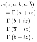
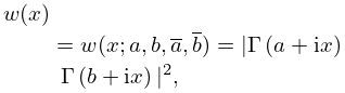
… ►A system of polynomials $\{{\varphi }_n(z)\}$, $n=0,1,\mathrm{\dots }$, where ${\varphi }_n(z)$ is of proper degree $n$, is orthonormal on the unit circle with respect to the weight function $w(z)$ ($\ge 0$) if … ►Let $\{p_n(x)\}$ and $\{q_n(x)\}$, $n=0,1,\mathrm{\dots }$, be OP’s with weight functions $w_1(x)$ and $w_2(x)$, respectively, on $(-1,1)$. … ►Instead of (18.33.9) one might take monic OP’s $\{q_n(x)\}$ with weight function $(1+x)w_1(x)$, and then express $q_n\left(\frac{1}{2}(z+z^{-1})\right)$ in terms of ${\varphi }_{2n}(z^{\pm 1})$ or ${\varphi }_{2n+1}(z^{\pm 1})$. … ►for some weight function $w(z)$ ($\ge 0$) then (18.33.17) (see also (18.33.1)) takes the form … ►For $w(z)$ as in (18.33.19) (or more generally as the weight function of the absolutely continuous part of the measure $\mu$ in (18.33.17)) and with ${\alpha }_n$ the Verblunsky coefficients in (18.33.23), (18.33.24), Szegő’s theorem states that …

12: 18.2 General Orthogonal Polynomials

… ►For OP’s $\{p_n(x)\}$ on $ℝ$ with respect to an even weight function $w(x)$ we have … ►This is the class of weight functions $w$ on $(-1,1)$ such that, in addition to (18.2.1_5), …Under further conditions on the weight function there is an equiconvergence theorem, see Szegő (1975, Theorem 13.1.2). … ►

Monotonic Weight Functions

… ► …

13: 18.19 Hahn Class: Definitions

… ►

Table 18.19.1: Orthogonality properties for Hahn, Krawtchouk, Meixner, and Charlier OP’s: discrete sets, weight functions, standardizations, and parameter constraints.

► ►►

	$p_n(x)$	$X$	$w_x$	$h_n$
…

►

… ►

18.19.2 $$w(z;a,b,\overline{a},\overline{b})=\mathrm{\Gamma }\left(a+iz\right)\mathrm{\Gamma }\left(b+iz\right)\mathrm{\Gamma }\left(\overline{a}-iz\right)\mathrm{\Gamma }\left(\overline{b}-iz\right),$$

ⓘ

Symbols:

$\mathrm{\Gamma }\left(z\right)$: gamma function, $\overline{z}$: complex conjugate, $w(x)$: weight function and $z$: complex variable

Permalink:

http://dlmf.nist.gov/18.19.E2

Encodings:

pMML, png, TeX

See also:

Annotations for §18.19, §18.19 and Ch.18

►

18.19.3 $$w(x)=w(x;a,b,\overline{a},\overline{b})={|\mathrm{\Gamma }\left(a+\mathrm{i}x\right)\mathrm{\Gamma }\left(b+\mathrm{i}x\right)|}^2,$$

ⓘ

Symbols:

$\mathrm{\Gamma }\left(z\right)$: gamma function, $\overline{z}$: complex conjugate, $\mathrm{i}$: imaginary unit, $w(x)$: weight function and $x$: real variable

Permalink:

http://dlmf.nist.gov/18.19.E3

Encodings:

pMML, png, TeX

See also:

Annotations for §18.19, §18.19 and Ch.18

… ►

18.19.7 $$w^{(\lambda )}(z;\varphi )=\mathrm{\Gamma }\left(\lambda +iz\right)\mathrm{\Gamma }\left(\lambda -iz\right){\mathrm{e}}^{(2\varphi -\pi )z},$$

ⓘ

Symbols:

$\mathrm{\Gamma }\left(z\right)$: gamma function, $\pi$: the ratio of the circumference of a circle to its diameter, $\mathrm{e}$: base of natural logarithm, $w(x)$: weight function and $z$: complex variable

Permalink:

http://dlmf.nist.gov/18.19.E7

Encodings:

pMML, png, TeX

See also:

Annotations for §18.19, §18.19 and Ch.18

…

14: 18.36 Miscellaneous Polynomials

… ►These are OP’s on the interval $(-1,1)$ with respect to an orthogonality measure obtained by adding constant multiples of “Dirac delta weights” at $-1$ and $1$ to the weight function for the Jacobi polynomials. … ►Orthogonality of the the classical OP’s with respect to a positive weight function, as in Table 18.3.1 requires, via Favard’s theorem, $A_n{A}_{n-1}{C}_n>0$ for $n\ge 1$ as per (18.2.9_5). … ►implying that, for $n\ge k$, the orthogonality of the $L_n^{(-k)}\left(x\right)$ with respect to the Laguerre weight function $x^{-k}{\mathrm{e}}^{-x}$, $x\in [0,\mathrm{\infty })$. … ►Consider the weight function … ►and orthonormal with respect to the weight function …

15: 3.11 Approximation Techniques

… ►

§3.11(iii) Minimax Rational Approximations

… ►Then the minimax (or best uniform) rational approximation … ► $w(x)$ being a given positive weight function, and again $J\ge n+1$. Then (3.11.29) is replaced by … ► …

16: 18.38 Mathematical Applications

… ►If the nodes in a quadrature formula with a positive weight function are chosen to be the zeros of the $n$th degree OP with the same weight function, and the interval of orthogonality is the same as the integration range, then the weights in the quadrature formula can be chosen in such a way that the formula is exact for all polynomials of degree not exceeding $2n-1$. … ►The basic ideas of Gaussian quadrature, and their extensions to non-classical weight functions, and the computation of the corresponding quadrature abscissas and weights, have led to discrete variable representations, or DVRs, of Sturm–Liouville and other differential operators. …Each of these typically require a particular non-classical weight functions and analysis of the corresponding OP’s. … ►Hermite polynomials (and their Freud-weight analogs (§18.32)) play an important role in random matrix theory. … ►

Non-Classical Weight Functions

…

17: Bibliography R

… ►

Erratum to:Relationships between the zeros, weights, and weight functions of orthogonal polynomials: Derivative rule approach to Stieltjes and spectral imaging. Computing in Science and Engineering 23 (4), pp. 91.

ⓘ

External Links:

ISSN 1521-9615, Document, Link

Referenced by:

§18.39(iv), §18.40(ii).

Encodings:

BibTeX

►

Relationships between the zeros, weights, and weight functions of orthogonal polynomials: Derivative rule approach to Stieltjes and spectral imaging. Computing in Science and Engineering 23 (3), pp. 56–64.

ⓘ

External Links:

ISSN 1521-9615, Document, Link

Referenced by:

§18.39(iv), §18.40(ii).

Encodings:

BibTeX

…

18: 31.9 Orthogonality

… ►

31.9.5 $${\int }_{{ℒ}_1}{\int }_{{ℒ}_2}\rho (s,t)w_1(s)w_1(t)w_2(s)w_2(t)dsdt=0,$$ $|n_1-n_2|+|m_1-m_2|\ne 0$,

ⓘ

Symbols:

$dx$: differential of $x$ , $\int$: integral, $m$: nonnegative integer, $n$: nonnegative integer, $\rho (s,t)$: weight function and ${ℒ}_1$, ${ℒ}_2$: integration paths

Permalink:

http://dlmf.nist.gov/31.9.E5

Encodings:

pMML, png, TeX

See also:

Annotations for §31.9(ii), §31.9 and Ch.31

… ►

31.9.6 $$\rho (s,t)=(s-t){(st)}^{\gamma -1}{\left((s-1)(t-1)\right)}^{\delta -1}{\left((s-a)(t-a)\right)}^{ϵ-1},$$

ⓘ

Defines:

$\rho (s,t)$: weight function (locally)

Symbols:

$\gamma$: real or complex parameter, $\delta$: real or complex parameter, $ϵ$: real or complex parameter and $a$: complex parameter

Permalink:

http://dlmf.nist.gov/31.9.E6

Encodings:

pMML, png, TeX

See also:

Annotations for §31.9(ii), §31.9 and Ch.31

…

19: 31.10 Integral Equations and Representations

… ►

31.10.1 $$W(z)={\int }_C𝒦(z,t)w(t)\rho (t)dt$$

ⓘ

Defines:

$W(z)$: solution (locally)

Symbols:

$dx$: differential of $x$ , $\int$: integral, $z$: complex variable, $C$: contour, $\rho (t)$: weight function and $𝒦(z,t)$: kernel

Referenced by:

§31.10(i), §31.10(i)

Permalink:

http://dlmf.nist.gov/31.10.E1

Encodings:

pMML, png, TeX

See also:

Annotations for §31.10(i), §31.10 and Ch.31

… ►The weight function is given by ►

31.10.2 $$\rho (t)=t^{\gamma -1}{(t-1)}^{\delta -1}{(t-a)}^{ϵ-1},$$

ⓘ

Defines:

$\rho (t)$: weight function (locally)

Symbols:

$\gamma$: real or complex parameter, $\delta$: real or complex parameter, $ϵ$: real or complex parameter and $a$: complex parameter

Permalink:

http://dlmf.nist.gov/31.10.E2

Encodings:

pMML, png, TeX

See also:

Annotations for §31.10(i), §31.10 and Ch.31

… ►The weight function is ►

31.10.13 $$\rho (s,t)=(s-t){(st)}^{\gamma -1}{\left((1-s)(1-t)\right)}^{\delta -1}{\left((1-(s/a))(1-(t/a))\right)}^{ϵ-1},$$

ⓘ

Defines:

$\rho (s,t)$: weight function (locally)

Symbols:

$\gamma$: real or complex parameter, $\delta$: real or complex parameter, $ϵ$: real or complex parameter and $a$: complex parameter

Permalink:

http://dlmf.nist.gov/31.10.E13

Encodings:

pMML, png, TeX

See also:

Annotations for §31.10(ii), §31.10 and Ch.31

…

20: 18.1 Notation

… ► ►►►►

$x,y,t$	real variables.
…
$w(x)$	weight function $(\ge 0)$ on an open interval $(a,b)$.
$w_x$	weights $(>0)$ at points $x\in X$ of a finite or countably infinite subset of $ℝ$.
…

…