type 2 Pollaczek polynomials counterexample

SearchAdvancedHelp

(0.006 seconds)

1—10 of 844 matching pages

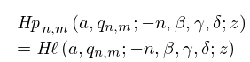
1: 31.5 Solutions Analytic at Three Singularities: Heun Polynomials

§31.5 Solutions Analytic at Three Singularities: Heun Polynomials

►Let $\alpha =-n$, $n=0,1,2,\mathrm{\dots }$, and $q_{n,m}$, $m=0,1,\mathrm{\dots },n$, be the eigenvalues of the tridiagonal matrix … ►

31.5.2 $${\mathrm{𝐻𝑝}}_{n,m}(a,q_{n,m};-n,\beta ,\gamma ,\delta ;z)=H\mathrm{\ell }(a,q_{n,m};-n,\beta ,\gamma ,\delta ;z)$$

ⓘ

Defines:

${\mathrm{𝐻𝑝}}_{n,m}(a,q_{n,m};-n,\beta ,\gamma ,\delta ;z)$: Heun polynomials

Symbols:

$H\mathrm{\ell }(a,q;\alpha ,\beta ,\gamma ,\delta ;z)$: Heun functions, $z$: complex variable, $\gamma$: real or complex parameter, $\delta$: real or complex parameter, $m$: nonnegative integer, $n$: nonnegative integer, $a$: complex parameter, $q$: real or complex parameter and $\beta$: real or complex parameter

Permalink:

http://dlmf.nist.gov/31.5.E2

Encodings:

pMML, png, TeX

See also:

Annotations for §31.5 and Ch.31

►is a polynomial of degree $n$, and hence a solution of (31.2.1) that is analytic at all three finite singularities $0,1,a$. These solutions are the Heun polynomials. …

2: 35.4 Partitions and Zonal Polynomials

§35.4 Partitions and Zonal Polynomials

… ►

Normalization

… ►

Orthogonal Invariance

… ►

Summation

►For $k=0,1,2,\mathrm{\dots }$, …

3: 24.1 Special Notation

… ►

Bernoulli Numbers and Polynomials

►The origin of the notation $B_n$, $B_n\left(x\right)$, is not clear. … ►

$B_2=\frac{1}{30}$ ,

… ►

Euler Numbers and Polynomials

… ►The notations $E_n$, $E_n\left(x\right)$, as defined in §24.2(ii), were used in Lucas (1891) and Nörlund (1924). …

4: 18.3 Definitions

§18.3 Definitions

… ►

With the property that ${\{p_{n+1}^{\prime }(x)\}}_{n=0}^{\mathrm{\infty }}$ is again a system of OP’s. See §18.9(iii).

… ►In addition to the orthogonal property given by Table 18.3.1, the Chebyshev polynomials $T_n\left(x\right)$, $n=0,1,\mathrm{\dots },N$, are orthogonal on the discrete point set comprising the zeros $x_{N+1,n},n=1,2,\mathrm{\dots },N+1$, of $T_{N+1}\left(x\right)$: … ►For $\nu \in ℝ$ and $N>-\frac{1}{2}$ a finite system of Jacobi polynomials $P_n^{(-N-1+\mathrm{i}\nu ,-N-1-\mathrm{i}\nu )}\left(\mathrm{i}x\right)$ (called pseudo Jacobi polynomials or Routh–Romanovski polynomials) is orthogonal on $(-\mathrm{\infty },\mathrm{\infty })$ with $w(x)={\left(1+x^2\right)}^{-N-1}{\mathrm{e}}^{2\nu \arctan x}$. … ►

Bessel polynomials

…

5: 18.35 Pollaczek Polynomials

… ► … ►we have the explicit representations … ► … … ►Then …

6: 18.30 Associated OP’s

… ►

§18.30(v) Associated Meixner–Pollaczek Polynomials

… ►They can be expressed in terms of type 3 Pollaczek polynomials (which are also associated type 2 Pollaczek polynomials) by (18.35.10). … ►The type 3 Pollaczek polynomials are the associated type 2 Pollaczek polynomials, see §18.35. The relationship (18.35.8) implies the definition for the associated ultraspherical polynomials $C_n^{(\lambda )}(x;c)=P_n^{(\lambda )}(x;0,0,c)$.

7: 27.19 Methods of Computation: Factorization

… ►Techniques for factorization of integers fall into three general classes: Deterministic algorithms, Type I probabilistic algorithms whose expected running time depends on the size of the smallest prime factor, and Type II probabilistic algorithms whose expected running time depends on the size of the number to be factored. … ►Type I probabilistic algorithms include the Brent–Pollard rho algorithm (also called Monte Carlo method), the Pollard $p-1$ algorithm, and the Elliptic Curve Method (ecm). … ►Type II probabilistic algorithms for factoring $n$ rely on finding a pseudo-random pair of integers $(x,y)$ that satisfy $x^2\equiv y^2(modn)$. …As of January 2009 the snfs holds the record for the largest integer that has been factored by a Type II probabilistic algorithm, a 307-digit composite integer. …The largest composite numbers that have been factored by other Type II probabilistic algorithms are a 63-digit integer by cfrac, a 135-digit integer by mpqs, and a 182-digit integer by gnfs. …

8: 18.39 Applications in the Physical Sciences

… ►The recursion of (18.39.46) is that for the type 2 Pollaczek polynomials of (18.35.2), with $\lambda =l+1$, $a=-b=2Z/s$, and $c=0$, and terminates for $x=x_i^N$ being a zero of the polynomial of order $N$. Thus the $c_N(x)=P_N^{(l+1)}(x;\frac{2Z}{s},-\frac{2Z}{s})$ and the eigenvalues …are determined by the $N$ zeros, $x_i^N$ of the Pollaczek polynomial $P_N^{(l+1)}(x;\frac{2Z}{s},-\frac{2Z}{s})$. ►

The Coulomb–Pollaczek Polynomials

►The polynomials $P_N^{(l+1)}(x;\frac{2Z}{s},-\frac{2Z}{s})$, for both positive and negative $Z$, define the Coulomb–Pollaczek polynomials (CP OP’s in what follows), see Yamani and Reinhardt (1975, Appendix B, and §IV). …

9: 10.64 Integral Representations

… ►

Schläfli-Type Integrals

►

10.64.1 $${\mathrm{ber}}_n\left(x\sqrt{2}\right)=\frac{{(-1)}^n}{\pi }{\int }_0^{\pi }\cos \left(x\sin t-nt\right)\cosh \left(x\sin t\right)dt,$$

ⓘ

Symbols:

${\mathrm{ber}}_{\nu }\left(x\right)$: Kelvin function, $\pi$: the ratio of the circumference of a circle to its diameter, $\cos z$: cosine function, $dx$: differential of $x$ , $\cosh z$: hyperbolic cosine function, $\int$: integral, $\sin z$: sine function, $n$: integer and $x$: real variable

Permalink:

http://dlmf.nist.gov/10.64.E1

Encodings:

pMML, png, TeX

See also:

Annotations for §10.64, §10.64 and Ch.10

►

10.64.2 $${\mathrm{bei}}_n\left(x\sqrt{2}\right)=\frac{{(-1)}^n}{\pi }{\int }_0^{\pi }\sin \left(x\sin t-nt\right)\sinh \left(x\sin t\right)dt.$$

ⓘ

Symbols:

${\mathrm{bei}}_{\nu }\left(x\right)$: Kelvin function, $\pi$: the ratio of the circumference of a circle to its diameter, $dx$: differential of $x$ , $\sinh z$: hyperbolic sine function, $\int$: integral, $\sin z$: sine function, $n$: integer and $x$: real variable

Permalink:

http://dlmf.nist.gov/10.64.E2

Encodings:

pMML, png, TeX

See also:

Annotations for §10.64, §10.64 and Ch.10

►See Apelblat (1991) for these results, and also for similar representations for ${\mathrm{ber}}_{\nu }\left(x\sqrt{2}\right)$, ${\mathrm{bei}}_{\nu }\left(x\sqrt{2}\right)$, and their $\nu$-derivatives. …

10: Bibliography P

… ►

A Kummer-type transformation for a ${}_2{}^{}F_2^{}$ hypergeometric function. J. Comput. Appl. Math. 173 (2), pp. 379–382.

ⓘ

External Links:

ISSN 0377-0427, Document, MathReview (P. Anandani), ZentralBlatt

Referenced by:

§16.6.

Encodings:

BibTeX

… ►

Sur une généralisation des polynomes de Legendre. C. R. Acad. Sci. Paris 228, pp. 1363–1365.

ⓘ

External Links:

ISSN 0001-4036, MathReview (G. Szegö)

Referenced by:

§18.35(i).

Encodings:

BibTeX

►

Systèmes de polynomes biorthogonaux qui généralisent les polynomes ultrasphériques. C. R. Acad. Sci. Paris 228, pp. 1998–2000.

ⓘ

External Links:

ISSN 0001-4036, MathReview (G. Szegö)

Referenced by:

§18.35(i).

Encodings:

BibTeX

►

Sur une famille de polynômes orthogonaux à quatre paramètres. C. R. Acad. Sci. Paris 230, pp. 2254–2256.

ⓘ

External Links:

MathReview (A. Erdélyi)

Referenced by:

(18.30.17), (18.30.18), (18.35.6_5), (18.35.6_6), §18.35(i).

Encodings:

BibTeX

… ►

Voronoi type congruences for Bernoulli numbers. In Voronoi’s Impact on Modern Science. Book I, P. Engel and H. Syta (Eds.),

ⓘ

External Links:

ZentralBlatt

Referenced by:

§24.10(iii).

Encodings:

BibTeX

…