…
►When a rigorous bound or reliable estimate for the remainder term is unavailable, it is unsafe to judge the accuracy of an asymptotic expansion merely from the numerical rate of decrease of the terms at the point of truncation.
…
►If the results agree within significant figures, then it is likely—but not certain—that the truncated asymptotic series will yield at least correct significant figures for larger values of .
…
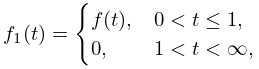
►Truncation after 5 terms yields 0.
…
►The process just used is equivalent to re-expanding the remainder term of the original asymptotic series (2.11.24) in powers of and truncating the new series optimally.
…
►Optimum truncation occurs just prior to the numerically smallest term, that is, at .
…
…
►Because the series (3.11.12) converges rapidly we obtain a very good first approximation to the minimax polynomial for if we truncate (3.11.12) at its th term.
…
►Since , is a monotonically increasing function of , and (for example) , this means that in practice the gain in replacing a truncated Chebyshev-series expansion by the corresponding minimax polynomial approximation is hardly worthwhile.
…
►Let be the last term retained in the truncated series.
…Then the sum of the truncated expansion equals .
…
…
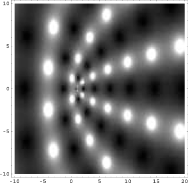
►►►Figure 22.3.26: Density plot of as a function of complex , , .
Grayscale, running from 0 (black) to 10 (white), with
truncated to 10.
…
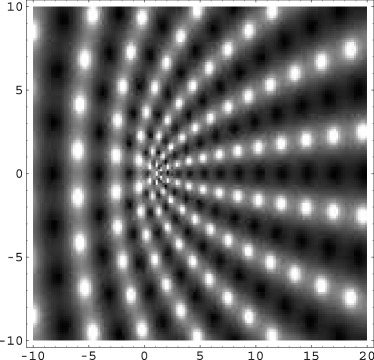
Magnify►►►Figure 22.3.27: Density plot of as a function of complex , , .
Grayscale, running from 0 (black) to 10 (white), with
truncated to 10.
…
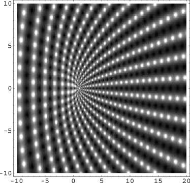
Magnify►►►Figure 22.3.28: Density plot of as a function of complex , , .
Grayscale, running from 0 (black) to 10 (white), with
truncated to 10.
…
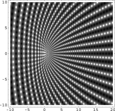
Magnify►►►Figure 22.3.29: Density plot of as a function of complex , , .
Grayscale, running from 0 (black) to 10 (white), with
truncated to 10.
…
Magnify
E. J. Weniger (2007)Asymptotic Approximations to Truncation Errors of Series Representations for Special Functions.
In Algorithms for Approximation, A. Iske and J. Levesley (Eds.),
pp. 331–348.
…
►Coefficients of terms up to are given in Lee (1990), along with tables of fractional errors in and , , obtained by using 12 different truncations of (19.5.6) in (19.5.8) and (19.5.9).
…
 ►
►
 ►
►
 ►
►
 ►
►
