relation to umbilics

SearchAdvancedHelp

(0.002 seconds)

5 matching pages

1: 36.2 Catastrophes and Canonical Integrals

… ►Addendum: For further special cases see §36.2(iv) …

2: 36.5 Stokes Sets

… ►Stokes sets are surfaces (codimension one) in $𝐱$ space, across which ${\mathrm{\Psi }}_K(𝐱;k)$ or ${\mathrm{\Psi }}^{(\mathrm{U})}(𝐱;k)$ acquires an exponentially-small asymptotic contribution (in $k$), associated with a complex critical point of ${\mathrm{\Phi }}_K$ or . … ►

§36.5(iii) Umbilics

►

Elliptic Umbilic Stokes Set (Codimension three)

►This consists of three separate cusp-edged sheets connected to the cusp-edged sheets of the bifurcation set, and related by rotation about the $z$-axis by $2\pi /3$. … ►

Hyperbolic Umbilic Stokes Set (Codimension three)

…

3: 36.7 Zeros

… ►

§36.7(iii) Elliptic Umbilic Canonical Integral

… ►The zeros are lines in $𝐱=(x,y,z)$ space where $\mathrm{ph}{\mathrm{\Psi }}^{(\mathrm{E})}\left(𝐱\right)$ is undetermined. …Outside the bifurcation set (36.4.10), each rib is flanked by a series of zero lines in the form of curly “antelope horns” related to the “outside” zeros (36.7.2) of the cusp canonical integral. … ►

§36.7(iv) Swallowtail and Hyperbolic Umbilic Canonical Integrals

►The zeros of these functions are curves in $𝐱=(x,y,z)$ space; see Nye (2007) for ${\mathrm{\Phi }}_3$ and Nye (2006) for ${\mathrm{\Phi }}^{(\mathrm{H})}$.

4: Errata

… ►

The Kronecker delta symbols have been moved furthest to the right, as is common convention for orthogonality relations.

… ►

Scales were corrected in all figures. The interval $-8.4\le \frac{x-y}{\sqrt{2}}\le 8.4$ was replaced by $-12.0\le \frac{x-y}{\sqrt{2}}\le 12.0$ and $-12.7\le \frac{x+y}{\sqrt{2}}\le 4.2$ replaced by $-18.0\le \frac{x+y}{\sqrt{2}}\le 6.0$. All plots and interactive visualizations were regenerated to improve image quality.

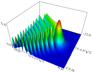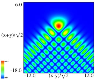
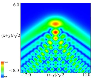
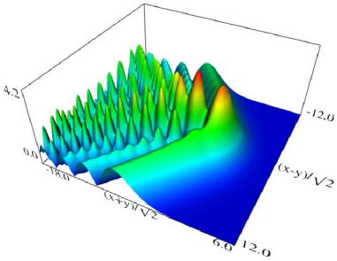
(a) Density plot.	(b) 3D plot.

Figure 36.3.9: Modulus of hyperbolic umbilic canonical integral function $|{\mathrm{\Psi }}^{(\mathrm{H})}\left(x,y,0\right)|$.

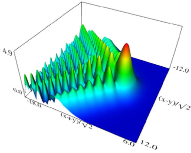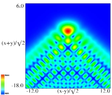
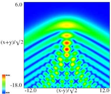
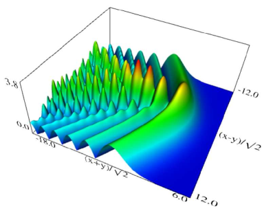
(a) Density plot.	(b) 3D plot.

Figure 36.3.10: Modulus of hyperbolic umbilic canonical integral function $|{\mathrm{\Psi }}^{(\mathrm{H})}\left(x,y,1\right)|$.

(a) Density plot.	(b) 3D plot.

Figure 36.3.11: Modulus of hyperbolic umbilic canonical integral function $|{\mathrm{\Psi }}^{(\mathrm{H})}\left(x,y,2\right)|$.

(a) Density plot.	(b) 3D plot.

Figure 36.3.12: Modulus of hyperbolic umbilic canonical integral function $|{\mathrm{\Psi }}^{(\mathrm{H})}\left(x,y,3\right)|$.

Reported 2016-09-12 by Dan Piponi.

►

The scaling error reported on 2016-09-12 by Dan Piponi also applied to contour and density plots for the phase of the hyperbolic umbilic canonical integrals. Scales were corrected in all figures. The interval $-8.4\le \frac{x-y}{\sqrt{2}}\le 8.4$ was replaced by $-12.0\le \frac{x-y}{\sqrt{2}}\le 12.0$ and $-12.7\le \frac{x+y}{\sqrt{2}}\le 4.2$ replaced by $-18.0\le \frac{x+y}{\sqrt{2}}\le 6.0$. All plots and interactive visualizations were regenerated to improve image quality.

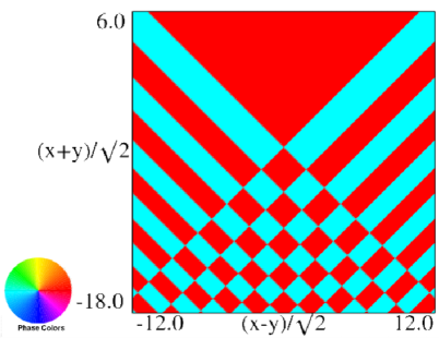(a) Contour plot.	(b) Density plot.

Figure 36.3.18: Phase of hyperbolic umbilic canonical integral $\mathrm{ph}{\mathrm{\Psi }}^{(\mathrm{H})}\left(x,y,0\right)$.

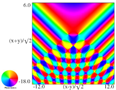(a) Contour plot.	(b) Density plot.

Figure 36.3.19: Phase of hyperbolic umbilic canonical integral $\mathrm{ph}{\mathrm{\Psi }}^{(\mathrm{H})}\left(x,y,1\right)$.

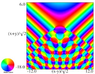(a) Contour plot.	(b) Density plot.

Figure 36.3.20: Phase of hyperbolic umbilic canonical integral $\mathrm{ph}{\mathrm{\Psi }}^{(\mathrm{H})}\left(x,y,2\right)$.

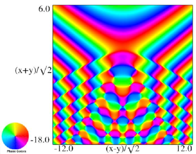(a) Contour plot.	(b) Density plot.

Figure 36.3.21: Phase of hyperbolic umbilic canonical integral $\mathrm{ph}{\mathrm{\Psi }}^{(\mathrm{H})}\left(x,y,3\right)$.

Reported 2016-09-28.

… ►

A number of additions and changes have been made to the metadata to reflect new and changed references as well as to how some equations have been derived.

… ►

36.10.14 $$3\left(\frac{{\partial }^2{\mathrm{\Psi }}^{(\mathrm{E})}}{{\partial x}^2}-\frac{{\partial }^2{\mathrm{\Psi }}^{(\mathrm{E})}}{{\partial y}^2}\right)+2\mathrm{i}z\frac{\partial {\mathrm{\Psi }}^{(\mathrm{E})}}{\partial x}-x{\mathrm{\Psi }}^{(\mathrm{E})}=0$$

Originally this equation appeared with $\frac{\partial {\mathrm{\Psi }}^{(\mathrm{H})}}{\partial x}$ in the second term, rather than $\frac{\partial {\mathrm{\Psi }}^{(\mathrm{E})}}{\partial x}$.

Reported 2010-04-02.

…

5: 36.12 Uniform Approximation of Integrals

… ►Define a mapping $u(t;𝐲)$ by relating $f(u;𝐲)$ to the normal form (36.2.1) of ${\mathrm{\Phi }}_K(t;𝐱)$ in the following way: … ►This technique can be applied to generate a hierarchy of approximations for the diffraction catastrophes ${\mathrm{\Psi }}_K(𝐱;k)$ in (36.2.10) away from $𝐱=\mathrm{𝟎}$, in terms of canonical integrals ${\mathrm{\Psi }}_J\left(\xi (𝐱;k)\right)$ for . For example, the diffraction catastrophe ${\mathrm{\Psi }}_2(x,y;k)$ defined by (36.2.10), and corresponding to the Pearcey integral (36.2.14), can be approximated by the Airy function ${\mathrm{\Psi }}_1\left(\xi (x,y;k)\right)$ when $k$ is large, provided that $x$ and $y$ are not small. … ►Also, ${\mathrm{\Delta }}^{1/4}/\sqrt{f_{+}^{\prime \prime }}$ and ${\mathrm{\Delta }}^{1/4}/\sqrt{-f_{-}^{\prime \prime }}$ are chosen to be positive real when $y$ is such that both critical points are real, and by analytic continuation otherwise. … ►For further information concerning integrals with several coalescing saddle points see Arnol’d et al. (1988), Berry and Howls (1993, 1994), Bleistein (1967), Duistermaat (1974), Ludwig (1966), Olde Daalhuis (2000), and Ursell (1972, 1980).