hyperbolic analog

SearchAdvancedHelp

(0.001 seconds)

5 matching pages

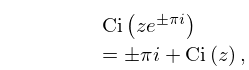
1: 6.4 Analytic Continuation

… ►

6.4.4 $$\mathrm{Ci}\left(z{\mathrm{e}}^{\pm \pi \mathrm{i}}\right)=\pm \pi \mathrm{i}+\mathrm{Ci}\left(z\right),$$

ⓘ

Symbols:

$\pi$: the ratio of the circumference of a circle to its diameter, $\mathrm{Ci}\left(z\right)$: cosine integral, $\mathrm{e}$: base of natural logarithm, $\mathrm{i}$: imaginary unit and $z$: complex variable

Referenced by:

§6.4

Permalink:

http://dlmf.nist.gov/6.4.E4

Encodings:

pMML, png, TeX

See also:

Annotations for §6.4 and Ch.6

…

2: 6.2 Definitions and Interrelations

… ►

Hyperbolic Analogs of the Sine and Cosine Integrals

…

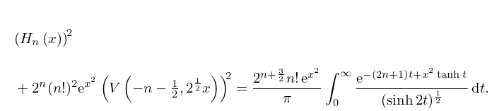
3: 18.17 Integrals

… ►For formulas for Jacobi and Laguerre polynomials analogous to (18.17.5) and (18.17.6), see Koornwinder (1974, 1977). … ►

18.17.8 $${\left(H_n\left(x\right)\right)}^2+2^n{(n!)}^2{\mathrm{e}}^{x^2}{\left(V(-n-\frac{1}{2},2^{\frac{1}{2}}x)\right)}^2=\frac{2^{n+\frac{3}{2}}n!{\mathrm{e}}^{x^2}}{\pi }{\int }_0^{\mathrm{\infty }}\frac{{\mathrm{e}}^{-(2n+1)t+x^2\tanh t}}{{(\sinh 2t)}^{\frac{1}{2}}}dt.$$

ⓘ

Symbols:

$H_n\left(x\right)$: Hermite polynomial, $\pi$: the ratio of the circumference of a circle to its diameter, $dx$: differential of $x$ , $\mathrm{e}$: base of natural logarithm, $!$: factorial (as in $n!$), $\sinh z$: hyperbolic sine function, $\tanh z$: hyperbolic tangent function, $\int$: integral, $V(a,z)$: parabolic cylinder function, $t$: real variable, $n$: nonnegative integer and $x$: real variable

Permalink:

http://dlmf.nist.gov/18.17.E8

Encodings:

pMML, png, TeX

See also:

Annotations for §18.17(iii), §18.17(iii), §18.17 and Ch.18

…

4: 10.20 Uniform Asymptotic Expansions for Large Order

… ►Note: Another way of arranging the above formulas for the coefficients $A_k(\zeta ),B_k(\zeta ),C_k(\zeta )$, and $D_k(\zeta )$ would be by analogy with (12.10.42) and (12.10.46). … ►

10.20.17 $$z=\pm {(\tau \coth \tau -{\tau }^2)}^{\frac{1}{2}}\pm \mathrm{i}{({\tau }^2-\tau \tanh \tau )}^{\frac{1}{2}},$$ $0\le \tau \le {\tau }_0$,

ⓘ

Symbols:

$\coth z$: hyperbolic cotangent function, $\tanh z$: hyperbolic tangent function, $\mathrm{i}$: imaginary unit and $z$: complex variable

Permalink:

http://dlmf.nist.gov/10.20.E17

Encodings:

pMML, png, TeX

See also:

Annotations for §10.20(ii), §10.20 and Ch.10

►where ${\tau }_0=1.19968\mathrm{\dots }$ is the positive root of the equation $\tau =\coth \tau$. …

5: 19.25 Relations to Other Functions

… ►

19.25.16 $$\mathrm{\Pi }(\varphi ,{\alpha }^2,k)=-\frac{1}{3}{\omega }^2{R}_J(c-1,c-k^2,c,c-{\omega }^2)+\sqrt{\frac{(c-1)(c-k^2)}{({\alpha }^2-1)(1-{\omega }^2)}}{R}_C(c({\alpha }^2-1)(1-{\omega }^2),({\alpha }^2-c)(c-{\omega }^2)),$$ ${\omega }^2=k^2/{\alpha }^2$.

ⓘ

Symbols:

$R_C(x,y)$: Carlson’s combination of inverse circular and inverse hyperbolic functions, $R_J(x,y,z,p)$: symmetric elliptic integral of third kind, $\mathrm{\Pi }(\varphi ,{\alpha }^2,k)$: Legendre’s incomplete elliptic integral of the third kind, $\varphi$: real or complex argument, $k$: real or complex modulus and ${\alpha }^2$: real or complex parameter

Referenced by:

§19.25(i)

Permalink:

http://dlmf.nist.gov/19.25.E16

Encodings:

pMML, png, TeX

See also:

Annotations for §19.25(i), §19.25 and Ch.19

… ►

19.25.30 $$\mathrm{am}(u,k)=R_C({\mathrm{cs}}^2(u,k),{\mathrm{ns}}^2(u,k)),$$

ⓘ

Symbols:

$R_C(x,y)$: Carlson’s combination of inverse circular and inverse hyperbolic functions, $\mathrm{am}(x,k)$: Jacobi’s amplitude function, $\mathrm{cs}(z,k)$: Jacobian elliptic function, $\mathrm{ns}(z,k)$: Jacobian elliptic function and $k$: real or complex modulus

Referenced by:

§19.25(v)

Permalink:

http://dlmf.nist.gov/19.25.E30

Encodings:

pMML, png, TeX

See also:

Annotations for §19.25(v), §19.25 and Ch.19

… ►For analogous integrals of the second kind, which are not invertible in terms of single-valued functions, see (19.29.20) and (19.29.21) and compare with Gradshteyn and Ryzhik (2000, §3.153,1–10 and §3.156,1–9). …