congruent points

SearchAdvancedHelp

(0.000 seconds)

11—20 of 156 matching pages

11: 10.72 Mathematical Applications

… ►

§10.72(i) Differential Equations with Turning Points

… ►

Simple Turning Points

… ►These expansions are uniform with respect to $z$, including the turning point $z_0$ and its neighborhood, and the region of validity often includes cut neighborhoods (§1.10(vi)) of other singularities of the differential equation, especially irregular singularities. … ►

Multiple or Fractional Turning Points

… ►

§10.72(iii) Differential Equations with a Double Pole and a Movable Turning Point

…

12: 33.23 Methods of Computation

… ►Inside the turning points, that is, when , there can be a loss of precision by a factor of approximately ${|G_{\mathrm{\ell }}|}^2$. … ►WKBJ approximations (§2.7(iii)) for $\rho >{\rho }_{\mathrm{tp}}(\eta ,\mathrm{\ell })$ are presented in Hull and Breit (1959) and Seaton and Peach (1962: in Eq. … ►Hull and Breit (1959) and Barnett (1981b) give WKBJ approximations for $F_0$ and $G_0$ in the region inside the turning point: .

13: 33.3 Graphics

… ►

►►

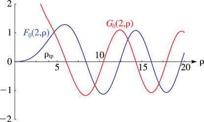
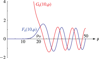
Figure 33.3.3: $F_{\mathrm{\ell }}(\eta ,\rho )$, $G_{\mathrm{\ell }}(\eta ,\rho )$ with $\mathrm{\ell }=0$, $\eta =2$. The turning point is at ${\rho }_{\mathrm{tp}}(2,0)=4$. Magnify

►

►►

Figure 33.3.4: $F_{\mathrm{\ell }}(\eta ,\rho )$, $G_{\mathrm{\ell }}(\eta ,\rho )$ with $\mathrm{\ell }=0$, $\eta =10$. The turning point is at ${\rho }_{\mathrm{tp}}(10,0)=20$. Magnify

… ►

►►

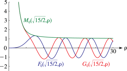
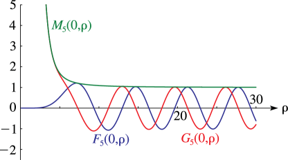
Figure 33.3.5: $F_{\mathrm{\ell }}(\eta ,\rho )$, $G_{\mathrm{\ell }}(\eta ,\rho )$, and $M_{\mathrm{\ell }}(\eta ,\rho )$ with $\mathrm{\ell }=0$, $\eta =\sqrt{15/2}$. The turning point is at ${\rho }_{\mathrm{tp}}(\sqrt{15/2},0)=\sqrt{30}=5.47\mathrm{\dots }$. Magnify

►

►►

Figure 33.3.6: $F_{\mathrm{\ell }}(\eta ,\rho )$, $G_{\mathrm{\ell }}(\eta ,\rho )$, and $M_{\mathrm{\ell }}(\eta ,\rho )$ with $\mathrm{\ell }=5$, $\eta =0$. The turning point is at ${\rho }_{\mathrm{tp}}(0,5)=\sqrt{30}$ (as in Figure 33.3.5). Magnify

…

14: 24.10 Arithmetic Properties

… ►Here and elsewhere two rational numbers are congruent if the modulus divides the numerator of their difference. …

15: 1.9 Calculus of a Complex Variable

… ►

§1.9(ii) Continuity, Point Sets, and Differentiation

… ►

Point Sets in $ℂ$

… ► … ►Points of a region that are not boundary points are called interior points. …

16: 23.20 Mathematical Applications

… ►For each pair of edges there is a unique point $z_0$ such that $\mathrm{\wp }\left(z_0\right)=0$. … ►Let $T$ denote the set of points on $C$ that are of finite order (that is, those points $P$ for which there exists a positive integer $n$ with $nP=o$), and let $I,K$ be the sets of points with integer and rational coordinates, respectively. …The resulting points are then tested for finite order as follows. …If any of these quantities is zero, then the point has finite order. If any of $2P$, $4P$, $8P$ is not an integer, then the point has infinite order. …

17: 4.48 Software

… ►All scientific programming languages, libraries, and systems support computation of at least some of the elementary functions in standard floating-point arithmetic (§3.1(i)). … ►A more complete list of available software for computing these functions is found in the Software Index; again, software that uses only standard floating-point arithmetic is excluded. …

18: 36.15 Methods of Computation

… ►Direct numerical evaluation can be carried out along a contour that runs along the segment of the real $t$-axis containing all real critical points of $\mathrm{\Phi }$ and is deformed outside this range so as to reach infinity along the asymptotic valleys of $\exp \left(\mathrm{i}\mathrm{\Phi }\right)$. … ►This can be carried out by direct numerical evaluation of canonical integrals along a finite segment of the real axis including all real critical points of $\mathrm{\Phi }$, with contributions from the contour outside this range approximated by the first terms of an asymptotic series associated with the endpoints. …

19: Bibliography Q

… ►

Uniform asymptotic expansions of a double integral: Coalescence of two stationary points. Proc. Roy. Soc. London Ser. A 456, pp. 407–431.

ⓘ

External Links:

ISSN 1364-5021, Document, MathReview (F. Ursell), ZentralBlatt

Referenced by:

§2.4(vi).

Encodings:

BibTeX

…

20: 2.4 Contour Integrals

… ►

§2.4(iv) Saddle Points

… ►

§2.4(v) Coalescing Saddle Points: Chester, Friedman, and Ursell’s Method

… ►

§2.4(vi) Other Coalescing Critical Points

… ►For a coalescing saddle point, a pole, and a branch point see Ciarkowski (1989). For many coalescing saddle points see §36.12. …