Racah polynomials

SearchAdvancedHelp

(0.002 seconds)

8 matching pages

1: 18.26 Wilson Class: Continued

… ►

18.26.4_2 $$R_n(y(y+\gamma +\delta +1);\alpha ,\beta ,\gamma ,\delta )=R_y(n(n+\alpha +\beta +1);\gamma ,\delta ,\alpha ,\beta ).$$

ⓘ

Symbols:

$R_n(x;\alpha ,\beta ,\gamma ,\delta )$: Racah polynomial, $y$: real variable, $\delta$: arbitrary small positive constant and $n$: nonnegative integer

Referenced by:

§18.26(i), Erratum (V1.2.0) Section 18.26

Permalink:

http://dlmf.nist.gov/18.26.E4_2

Encodings:

pMML, png, TeX

Addition (effective with 1.2.0):

This equation was added.

See also:

Annotations for §18.26(i), §18.26(i), §18.26 and Ch.18

… ►

18.26.9 $$\underset{\beta \to \mathrm{\infty }}{lim}{R}_n(x;-N-1,\beta ,\gamma ,\delta )=R_n(x;\gamma ,\delta ,N).$$

ⓘ

Symbols:

$R_n(x;\alpha ,\beta ,\gamma ,\delta )$: Racah polynomial, $R_n(x;\gamma ,\delta ,N)$: dual Hahn polynomial, $N$: positive integer, $\delta$: arbitrary small positive constant, $n$: nonnegative integer and $x$: real variable

Referenced by:

§18.26(ii)

Permalink:

http://dlmf.nist.gov/18.26.E9

Encodings:

pMML, png, TeX

See also:

Annotations for §18.26(ii), §18.26(ii), §18.26 and Ch.18

… ►

18.26.10 $$\underset{\delta \to \mathrm{\infty }}{lim}{R}_n(x(x+\gamma +\delta +1);\alpha ,\beta ,-N-1,\delta )=Q_n(x;\alpha ,\beta ,N).$$

ⓘ

Symbols:

$Q_n(x;\alpha ,\beta ,N)$: Hahn polynomial, $R_n(x;\alpha ,\beta ,\gamma ,\delta )$: Racah polynomial, $N$: positive integer, $\delta$: arbitrary small positive constant, $n$: nonnegative integer and $x$: real variable

Referenced by:

§18.26(ii)

Permalink:

http://dlmf.nist.gov/18.26.E10

Encodings:

pMML, png, TeX

See also:

Annotations for §18.26(ii), §18.26(ii), §18.26 and Ch.18

… ►

18.26.16 $$\frac{{\mathrm{\Delta }}_y\left(R_n(y(y+\gamma +\delta +1);\alpha ,\beta ,\gamma ,\delta )\right)}{{\mathrm{\Delta }}_y\left(y(y+\gamma +\delta +1)\right)}=\frac{n(n+\alpha +\beta +1)}{(\alpha +1)(\beta +\delta +1)(\gamma +1)}{R}_{n-1}(y(y+\gamma +\delta +2);\alpha +1,\beta +1,\gamma +1,\delta ).$$

ⓘ

Symbols:

$R_n(x;\alpha ,\beta ,\gamma ,\delta )$: Racah polynomial, $\mathrm{\Delta }$: forward difference operator, $y$: real variable, $\delta$: arbitrary small positive constant and $n$: nonnegative integer

Referenced by:

§16.4(iii)

Permalink:

http://dlmf.nist.gov/18.26.E16

Encodings:

pMML, png, TeX

See also:

Annotations for §18.26(iii), §18.26 and Ch.18

… ►Koornwinder (2009) rescales and reparametrizes Racah polynomials and Wilson polynomials in such a way that they are continuous in their four parameters, provided that these parameters are nonnegative. …

2: 18.25 Wilson Class: Definitions

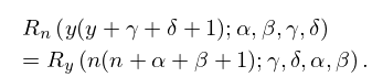
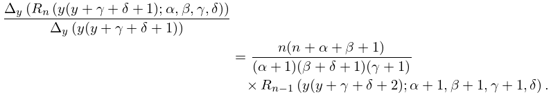
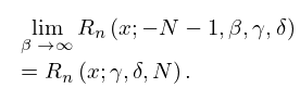
… ►Table 18.25.1 lists the transformations of variable, orthogonality ranges, and parameter constraints that are needed in §18.2(i) for the Wilson polynomials $W_n(x;a,b,c,d)$, continuous dual Hahn polynomials $S_n(x;a,b,c)$, Racah polynomials $R_n(x;\alpha ,\beta ,\gamma ,\delta )$, and dual Hahn polynomials $R_n(x;\gamma ,\delta ,N)$. ►

Table 18.25.1: Wilson class OP’s: transformations of variable, orthogonality ranges, and parameter constraints.

► ►►►

OP	$p_n(x)$	$x=\lambda (y)$	Orthogonality range for $y$	Constraints
…
Racah	$R_n(x;\alpha ,\beta ,\gamma ,\delta )$	$y(y+\gamma +\delta +1)$	$\{0,1,\mathrm{\dots },N\}$	$\alpha +1$ or $\beta +\delta +1$ or $\gamma +1=-N;$ for further constraints see (18.25.1)
…

►

… ►

Further Constraints for Racah Polynomials

… ►

18.25.10 $$p_n(x)=R_n(x;\alpha ,\beta ,\gamma ,\delta ),$$ $\alpha +1=-N$,

ⓘ

Symbols:

$R_n(x;\alpha ,\beta ,\gamma ,\delta )$: Racah polynomial, $N$: positive integer, $\delta$: arbitrary small positive constant, $p_n(x)$: polynomial of degree $n$ , $n$: nonnegative integer and $x$: real variable

Referenced by:

§18.25(iii)

Permalink:

http://dlmf.nist.gov/18.25.E10

Encodings:

pMML, png, TeX

See also:

Annotations for §18.25(iii), §18.25(iii), §18.25 and Ch.18

… ►

Table 18.25.2: Wilson class OP’s: leading coefficients.

► ►►►

$p_n(x)$	$k_n$
…
$R_n(x;\alpha ,\beta ,\gamma ,\delta )$	${\displaystyle \frac{{\left(n+\alpha +\beta +1\right)}_n}{{\left(\alpha +1\right)}_n{\left(\beta +\delta +1\right)}_n{\left(\gamma +1\right)}_n}}$
…

►

3: 18.28 Askey–Wilson Class

… ►Both the Askey–Wilson polynomials and the $q$-Racah polynomials can best be described as functions of $z$ (resp. … ►

§18.28(viii) $q$-Racah Polynomials

… ►

18.28.23 $$R_n(q^{-y}+\gamma \delta q^{y+1};\alpha ,\beta ,\gamma ,\delta |q)=R_y(q^{-n}+\alpha \beta q^{n+1};\gamma ,\delta ,\alpha ,\beta |q),$$ $\alpha q$, $\beta \delta q$, or $\gamma q=q^{-N}$; $n,y=0,1,\mathrm{\dots },N$.

ⓘ

Symbols:

$R_n(x;\alpha ,\beta ,\gamma ,\delta |q)$: $q$-Racah polynomial, $y$: real variable, $N$: positive integer, $\delta$: arbitrary small positive constant, $q$: real variable and $n$: nonnegative integer

Referenced by:

§18.28(viii), §18.28(viii), Erratum (V1.2.0) Section 18.28

Permalink:

http://dlmf.nist.gov/18.28.E23

Encodings:

pMML, png, TeX

See also:

Annotations for §18.28(viii), §18.28(viii), §18.28 and Ch.18

… ►These systems are the $q$-Racah polynomials and its limit cases. … ►

18.28.34 $$\underset{q\to 1}{lim}{R}_n(q^{-y}+q^{y+\gamma +\delta +1};q^{\alpha },q^{\beta },q^{\gamma },q^{\delta }|q)=R_n(y(y+\gamma +\delta +1);\alpha ,\beta ,\gamma ,\delta ).$$

ⓘ

Symbols:

$R_n(x;\alpha ,\beta ,\gamma ,\delta )$: Racah polynomial, $R_n(x;\alpha ,\beta ,\gamma ,\delta |q)$: $q$-Racah polynomial, $y$: real variable, $\delta$: arbitrary small positive constant, $q$: real variable and $n$: nonnegative integer

Source:

Koekoek et al. (2010, (14.2.24))

Referenced by:

§18.28(x), Erratum (V1.2.0) Section 18.28

Permalink:

http://dlmf.nist.gov/18.28.E34

Encodings:

pMML, png, TeX

See also:

Annotations for §18.28(x), §18.28(x), §18.28 and Ch.18

…

4: 18.1 Notation

… ►

$${(z_1,\mathrm{\dots },z_k;q)}_{\mathrm{\infty }}={(z_1;q)}_{\mathrm{\infty }}\mathrm{\cdots }{(z_k;q)}_{\mathrm{\infty }}.$$

… ►

Racah: $R_n(x;\alpha ,\beta ,\gamma ,\delta )$.

… ►

$q$-Racah: $R_n(x;\alpha ,\beta ,\gamma ,\delta |q)$.

…

5: 18.38 Mathematical Applications

… ►

Coding Theory

►For applications of Krawtchouk polynomials $K_n(x;p,N)$ and $q$-Racah polynomials $R_n(x;\alpha ,\beta ,\gamma ,\delta |q)$ to coding theory see Bannai (1990, pp. 38–43), Leonard (1982), and Chihara (1987). … ►The $6j$ symbol (34.4.3), with an alternative expression as a terminating balanced ${}_4{}^{}F_3^{}$ of unit argument, can be expressend in terms of Racah polynomials (18.26.3). The orthogonality relations (34.5.14) for the $6j$ symbols can be rewritten in terms of orthogonality relations for Racah polynomials as given by (18.25.9)–(18.25.12). … …

6: 16.4 Argument Unity

… ►One example of such a three-term relation is the recurrence relation (18.26.16) for Racah polynomials. … …

7: 18.21 Hahn Class: Interrelations

… ►

►►

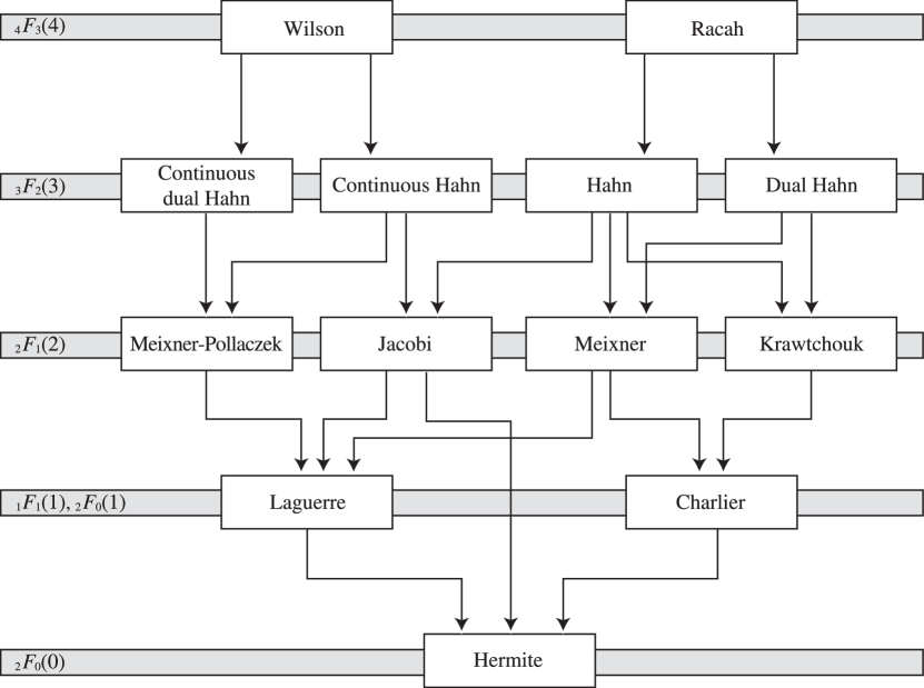
Figure 18.21.1: Askey scheme. …It increases by one for each row ascended in the scheme, culminating with four free real parameters for the Wilson and Racah polynomials. … Magnify

8: Bibliography C

… ►

Asymptotics of Racah coefficients and polynomials. J. Phys. A 32 (3), pp. 537–553.

ⓘ

External Links:

ISSN 0305-4470, Document, MathReview, ZentralBlatt

Referenced by:

§34.8, §34.8.

Encodings:

BibTeX

…