Jacobian
(0.002 seconds)
11—20 of 56 matching pages
11: 22.5 Special Values
§22.5 Special Values
… ►Table 22.5.1 gives the value of each of the 12 Jacobian elliptic functions, together with its -derivative (or at a pole, the residue), for values of that are integer multiples of , . … ► ►§22.5(ii) Limiting Values of
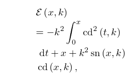
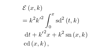
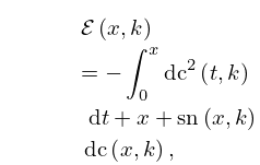
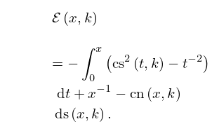
… ►12: 22.13 Derivatives and Differential Equations
…
►
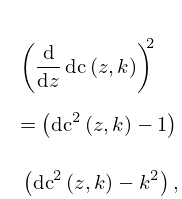
§22.13(i) Derivatives
► … ►§22.13(ii) First-Order Differential Equations
… ►
22.13.7
…
►
§22.13(iii) Second-Order Differential Equations
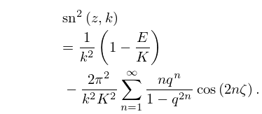
…13: 22.10 Maclaurin Series
…
►
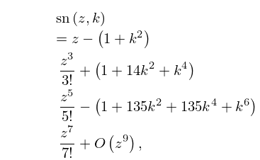
§22.10(i) Maclaurin Series in
… ►
22.10.1
…
►
§22.10(ii) Maclaurin Series in and
… ►
22.10.6
…
►
14: 22 Jacobian Elliptic Functions
Chapter 22 Jacobian Elliptic Functions
…15: 22.3 Graphics
…
►
►
 ►
►
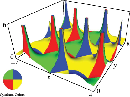
Figure 22.3.24:
for , , .
…
Magnify
3D
Help
►
►
 ►
►
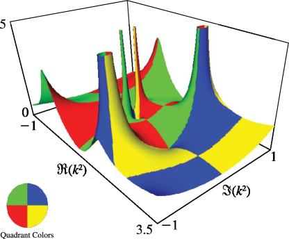
Figure 22.3.25:
as a function of complex , , .
…
Magnify
3D
Help
…
§22.3(i) Real Variables: Line Graphs
… ►§22.3(iii) Complex ; Real
… ►§22.3(iv) Complex
… ►
16: 22.19 Physical Applications
…
►
§22.19(ii) Classical Dynamics: The Quartic Oscillator
… ►§22.19(iii) Nonlinear ODEs and PDEs
… ►§22.19(iv) Tops
… ►§22.19(v) Other Applications
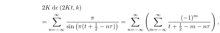
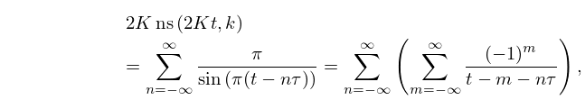
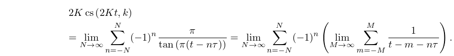
… ►17: 22.12 Expansions in Other Trigonometric Series and Doubly-Infinite Partial Fractions: Eisenstein Series
§22.12 Expansions in Other Trigonometric Series and Doubly-Infinite Partial Fractions: Eisenstein Series
… ►
22.12.2
…
►
22.12.8
…
►
22.12.11
…
►
22.12.13
18: Sidebar 22.SB1: Decay of a Soliton in a Bose–Einstein Condensate
…
►Jacobian elliptic functions arise as solutions to certain nonlinear Schrödinger equations, which model many types of wave propagation phenomena.
…
19: 22.11 Fourier and Hyperbolic Series
§22.11 Fourier and Hyperbolic Series
… ►In (22.11.7)–(22.11.12) the left-hand sides are replaced by their limiting values at the poles of the Jacobian functions. … ►
22.11.13
…
►A related hyperbolic series is
…
