.2022世界杯中国男足蠃_『welcom_』世界杯冠军加多少分_w2n3c1o_2022年12月10日16时49分8秒_zwuzf2w8s

SearchAdvancedHelp

The terms ".2022", "zwuzf2w8", "w2n3c1o" were not found.Possible alternative term: "2022".

(0.005 seconds)

1—10 of 355 matching pages

1: 11 Struve and Related Functions

…

2: 25.20 Approximations

… ►

Piessens and Branders (1972) gives the coefficients of the Chebyshev-series expansions of $s\zeta \left(s+1\right)$ and $\zeta \left(s+k\right)$, $k=2,3,4,5,8$, for $0\le s\le 1$ (23D).

… ►

Antia (1993) gives minimax rational approximations for $\mathrm{\Gamma }\left(s+1\right)F_s(x)$, where $F_s(x)$ is the Fermi–Dirac integral (25.12.14), for the intervals and , with $s=-\frac{1}{2},\frac{1}{2},\frac{3}{2},\frac{5}{2}$. For each $s$ there are three sets of approximations, with relative maximum errors ${10}^{-4},{10}^{-8},{10}^{-12}$.

3: Staff

… ►

Leonard C. Maximon, George Washington University, Chaps. 10, 34

… ►

Frank W. J. Olver, University of Maryland and NIST, Chaps. 1, 2, 4, 9, 10

… ►

Nico M. Temme, Centrum Wiskunde Informatica, Chaps. 3, 6, 7, 12

… ►

Diego Dominici, State University of New York at New Paltz, for Chaps. 9, 10 (deceased)

… ►

Nico M. Temme, Centrum Wiskunde & Informatica (CWI), for Chaps. 3, 6, 7, 12

…

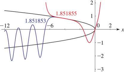
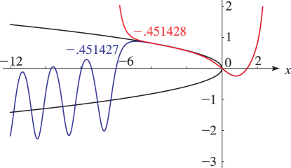
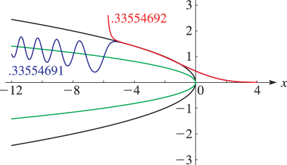
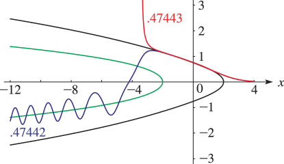
4: 32.3 Graphics

… ►

►►

Figure 32.3.3: $w_k(x)$ for $-12\le x\le 0.73$ and $k=\mathrm{1.85185\hspace{0.33em}3}$, $\mathrm{1.85185\hspace{0.33em}5}$. … Magnify

►

►►

Figure 32.3.4: $w_k(x)$ for $-12\le x\le 2.3$ and $k=-\mathrm{0.45142\hspace{0.33em}7}$, $-\mathrm{0.45142\hspace{0.33em}8}$. … Magnify

… ►

►►

Figure 32.3.7: $u_k(x;-\frac{1}{2})$ for $-12\le x\le 4$ with $k=\mathrm{0.33554\hspace{0.33em}691}$, $\mathrm{0.33554\hspace{0.33em}692}$. … Magnify

►

►►

Figure 32.3.8: $u_k(x;\frac{1}{2})$ for $-12\le x\le 4$ with $k=0.47442$, $0.47443$. … Magnify

►

►►

Figure 32.3.9: $u_k(x;\frac{3}{2})$ for $-12\le x\le 4$ with $k=0.38736$, $0.38737$. … Magnify

…

5: 12 Parabolic Cylinder Functions

Chapter 12 Parabolic Cylinder Functions

…

6: 27.2 Functions

… ►

Table 27.2.2: Functions related to division.

► ►►►►►►►

$n$	$\varphi \left(n\right)$	$d\left(n\right)$	$\sigma \left(n\right)$	$n$	$\varphi \left(n\right)$	$d\left(n\right)$	$\sigma \left(n\right)$	$n$	$\varphi \left(n\right)$	$d\left(n\right)$	$\sigma \left(n\right)$	$n$	$\varphi \left(n\right)$	$d\left(n\right)$	$\sigma \left(n\right)$
…
2	1	2	3	15	8	4	24	28	12	6	56	41	40	2	42
3	2	2	4	16	8	5	31	29	28	2	30	42	12	8	96
…
8	4	4	15	21	12	4	32	34	16	4	54	47	46	2	48
…
10	4	4	18	23	22	2	24	36	12	9	91	49	42	3	57
11	10	2	12	24	8	8	60	37	36	2	38	50	20	6	93
…

►

7: 24.2 Definitions and Generating Functions

… ►

Table 24.2.1: Bernoulli and Euler numbers.

► ►►►

$n$	$B_n$	$E_n$
…
$12$	$-\frac{691}{2730}$	$\mathrm{27\hspace{0.33em}02765}$
…

►

… ►

Table 24.2.3: Bernoulli numbers $B_n=N/D$.

► ►►►

$n$	$N$	$D$	$B_n$
…
$12$	$-691$	$2730$	$-\mathrm{2.53113\hspace{0.33em}5531}$	$\mathrm{\times 10⁻¹}$
…

►

►

Table 24.2.4: Euler numbers $E_n$.

► ►►►

$n$	$E_n$
…
$12$	$\mathrm{27\hspace{0.33em}02765}$
…

►

►

Table 24.2.5: Coefficients $b_{n,k}$ of the Bernoulli polynomials $B_n\left(x\right)={\sum }_{k=0}^n{b}_{n,k}{x}^k$.

► ►►►

	$k$
$n$	$0$	$1$	$2$	$3$	$4$	$5$	$6$	$7$	$8$	$9$	$10$	$11$	$12$	$13$	$14$	$15$
…

►

►

Table 24.2.6: Coefficients $e_{n,k}$ of the Euler polynomials $E_n\left(x\right)={\sum }_{k=0}^n{e}_{n,k}{x}^k$.

► ►►►

	$k$
$n$	$0$	$1$	$2$	$3$	$4$	$5$	$6$	$7$	$8$	$9$	$10$	$11$	$12$	$13$	$14$	$15$
…

►

8: 18.8 Differential Equations

… ►

Table 18.8.1: Classical OP’s: differential equations $A(x)f^{\prime \prime }(x)+B(x)f^{\prime }(x)+C(x)f(x)+{\lambda }_{n}f(x)=0$.

► ►►►►►

#	$f(x)$	$A(x)$	$B(x)$	$C(x)$	${\lambda }_n$
…
8	$L_n^{(\alpha )}\left(x\right)$	$x$	$\alpha +1-x$	$0$	$n$
…
10	${\mathrm{e}}^{-\frac{1}{2}x}{x}^{\frac{1}{2}\alpha }{L}_n^{(\alpha )}\left(x\right)$	$x$	$1$	$-\frac{1}{4}x-\frac{1}{4}{\alpha }^2{x}^{-1}$	$n+\frac{1}{2}(\alpha +1)$
…
12	$H_n\left(x\right)$	$1$	$-2x$	$0$	$2n$
…

►

…

9: 8.26 Tables

… ►

Zhang and Jin (1996, Table 3.9) tabulates $I_x(a,b)$ for $x=0(.05)1$, $a=0.5,1,3,5,10$, $b=1,10$ to 8D.

… ►

Abramowitz and Stegun (1964, pp. 245–248) tabulates $E_n\left(x\right)$ for $n=2,3,4,10,20$, $x=0(.01)2$ to 7D; also $(x+n){\mathrm{e}}^x{E}_n\left(x\right)$ for $n=2,3,4,10,20$, $x^{-1}=0(.01)0.1(.05)0.5$ to 6S.

… ►

Pagurova (1961) tabulates $E_n\left(x\right)$ for $n=0(1)20$, $x=0(.01)2(.1)10$ to 4-9S; ${\mathrm{e}}^x{E}_n\left(x\right)$ for $n=2(1)10$, $x=10(.1)20$ to 7D; ${\mathrm{e}}^x{E}_p\left(x\right)$ for $p=0(.1)1$, $x=0.01(.01)7(.05)12(.1)20$ to 7S or 7D.

►

Stankiewicz (1968) tabulates $E_n\left(x\right)$ for $n=1(1)10$, $x=0.01(.01)5$ to 7D.

►

Zhang and Jin (1996, Table 19.1) tabulates $E_n\left(x\right)$ for $n=1,2,3,5,10,15,20$, $x=0(.1)1,1.5,2,3,5,10,20,30,50,100$ to 7D or 8S.

10: 26.6 Other Lattice Path Numbers

… ►

Table 26.6.1: Delannoy numbers $D(m,n)$.

► ►►►►►

$m$	$n$
	0	1	2	3	4	5	6	7	8	9	10
…
8	1	17	145	833	3649	13073	40081	1 08545	2 65729	5 98417	12 56465
…
10	1	21	221	1561	8361	36365	1 34245	4 33905	12 56465	33 17445	80 97453

►

… ►

Table 26.6.2: Motzkin numbers $M(n)$.

► ►►►

$n$	$M(n)$	$n$	$M(n)$	$n$	$M(n)$	$n$	$M(n)$	$n$	$M(n)$
0	1	4	9	8	323	12	15511	16	8 53467
…

►

… ►

Table 26.6.4: Schröder numbers $r(n)$.

► ►►►

$n$	$r(n)$	$n$	$r(n)$	$n$	$r(n)$	$n$	$r(n)$	$n$	$r(n)$
$0$	$1$	$4$	$90$	$8$	$41586$	$12$	$\mathrm{272\hspace{0.33em}97738}$	$16$	$\mathrm{2\hspace{0.33em}09271\hspace{0.33em}56706}$
…

►

…