with respect to modulus

SearchAdvancedHelp

(0.012 seconds)

11—20 of 223 matching pages

11: 14.15 Uniform Asymptotic Approximations

… ►The points $x={\left(1-{\alpha }^2\right)}^{1/2}$, $x=1$, and $x=\mathrm{\infty }$ are mapped to $y={\alpha }^2$, $y=0$, and $y=-\mathrm{\infty }$, respectively. … ►uniformly with respect to $x\in (-1,1)$ and $\mu \in [\nu +\frac{1}{2},(1/\delta )(\nu +\frac{1}{2})]$. …

12: 32.7 Bäcklund Transformations

… ►

32.7.3 $$W(\zeta ;\frac{1}{2}\epsilon )=\frac{2^{-1/3}\epsilon }{w(z;0)}\frac{d}{dz}w(z;0),$$

ⓘ

Symbols:

$\frac{df}{dx}$: derivative of $f$ with respect to $x$ , $z$: real, $W(\zeta ,\epsilon /2)$: transformation and $\epsilon =\pm 1$

Permalink:

http://dlmf.nist.gov/32.7.E3

Encodings:

pMML, png, TeX

See also:

Annotations for §32.7(ii), §32.7 and Ch.32

… ►

32.7.4 $$w^2(z;0)=2^{-1/3}\left(W^2(\zeta ;\frac{1}{2}\epsilon )-\epsilon \frac{d}{d\zeta }W(\zeta ;\frac{1}{2}\epsilon )+\frac{1}{2}\zeta \right),$$

ⓘ

Symbols:

$\frac{df}{dx}$: derivative of $f$ with respect to $x$ , $z$: real, $W(\zeta ,\epsilon /2)$: transformation and $\epsilon =\pm 1$

Permalink:

http://dlmf.nist.gov/32.7.E4

Encodings:

pMML, png, TeX

See also:

Annotations for §32.7(ii), §32.7 and Ch.32

…

13: 9.8 Modulus and Phase

§9.8 Modulus and Phase

… ►(These definitions of $\theta \left(x\right)$ and $\varphi \left(x\right)$ differ from Abramowitz and Stegun (1964, Chapter 10), and agree more closely with those used in Miller (1946) and Olver (1997b, Chapter 11).) … ►Primes denote differentiations with respect to $x$, which is continued to be assumed real and nonpositive. … ►As $x$ increases from $-\mathrm{\infty }$ to $0$ each of the functions $M\left(x\right)$, $M^{\prime }\left(x\right)$, ${|x|}^{-1/4}N\left(x\right)$, $M\left(x\right)N\left(x\right)$, ${\theta }^{\prime }\left(x\right)$, ${\varphi }^{\prime }\left(x\right)$ is increasing, and each of the functions ${|x|}^{1/4}M\left(x\right)$, $\theta \left(x\right)$, $\varphi \left(x\right)$ is decreasing. … ►

14: 23.22 Methods of Computation

… ►The functions $\zeta \left(z\right)$ and $\sigma \left(z\right)$ are computed in a similar manner: the former by replacing $u$ and $z$ in (23.6.13) by $z$ and $\pi z/(2{\omega }_1)$, respectively, and also referring to (23.6.8); the latter by applying (23.6.9). … ►

In the general case, given by $cd\ne 0$, we compute the roots $\alpha$, $\beta$, $\gamma$, say, of the cubic equation $4t^3-ct-d=0$; see §1.11(iii). These roots are necessarily distinct and represent $e_1$, $e_2$, $e_3$ in some order.

If $c$ and $d$ are real, and the discriminant is positive, that is $c^3-27d^2>0$, then $e_1$, $e_2$, $e_3$ can be identified via (23.5.1), and $k^2$, $k_{}^{\prime }{}_{}{}^2$ obtained from (23.6.16).

If , or $c$ and $d$ are not both real, then we label $\alpha$, $\beta$, $\gamma$ so that the triangle with vertices $\alpha$, $\beta$, $\gamma$ is positively oriented and $[\alpha ,\gamma ]$ is its longest side (chosen arbitrarily if there is more than one). In particular, if $\alpha$, $\beta$, $\gamma$ are collinear, then we label them so that $\beta$ is on the line segment $(\alpha ,\gamma )$. In consequence, $k^2=(\beta -\gamma )/(\alpha -\gamma )$, $k_{}^{\prime }{}_{}{}^2=(\alpha -\beta )/(\alpha -\gamma )$ satisfy $\mathrm{\Im }{k}^2\ge 0\ge \mathrm{\Im }k_{}^{\prime }{}_{}{}^2$ (with strict inequality unless $\alpha$, $\beta$, $\gamma$ are collinear); also $|k^2|$, $|k_{}^{\prime }{}_{}{}^2|\le 1$.

Finally, on taking the principal square roots of $k^2$ and $k_{}^{\prime }{}_{}{}^2$ we obtain values for $k$ and $k^{\prime }$ that lie in the 1st and 4th quadrants, respectively, and $2{\omega }_1$, $2{\omega }_3$ are given by

23.22.1 $$2{\omega }_{1}M(1,k^{\prime })=-2\mathrm{i}{\omega }_{3}M(1,k)=\frac{\pi }{3}\sqrt{\frac{c(2+k^{2}k_{}^{\prime }{}_{}{}^2)(k_{}^{\prime }{}_{}{}^2-k^2)}{d(1-k^{2}k_{}^{\prime }{}_{}{}^2)}},$$

ⓘ

Symbols:

$M(a,g)$: arithmetic-geometric mean, $\pi$: the ratio of the circumference of a circle to its diameter, $\mathrm{i}$: imaginary unit, ${\omega }_1$, ${\omega }_3$, ${\omega }_2=-{\omega }_1-{\omega }_3$: lattice generators, $k$: modulus and $k^{\prime }$: complementary modulus

Proof sketch:

Combine (23.6.16), (23.6.17), (22.20.6), (23.3.5)–(23.3.7), and use analytical continuation.

Referenced by:

§23.22(ii)

Permalink:

http://dlmf.nist.gov/23.22.E1

Encodings:

pMML, png, TeX

See also:

Annotations for §23.22(ii), §23.22(ii), §23.22 and Ch.23

where $M$ denotes the arithmetic-geometric mean (see §§19.8(i) and 22.20(ii)). This process yields 2 possible pairs ($2{\omega }_1$, $2{\omega }_3$), corresponding to the 2 possible choices of the square root.

…

15: 22.16 Related Functions

… ►

22.16.30 $$ℰ(x,k)=\frac{1}{{\theta }_3^2(0,q){\theta }_4(\xi ,q)}\frac{d}{d\xi }{\theta }_4(\xi ,q)+\frac{E\left(k\right)}{K\left(k\right)}x,$$

ⓘ

Symbols:

$ℰ(x,k)$: Jacobi’s epsilon function, ${\theta }_j(z,q)$: theta function, $K\left(k\right)$: Legendre’s complete elliptic integral of the first kind, $E\left(k\right)$: Legendre’s complete elliptic integral of the second kind, $\frac{df}{dx}$: derivative of $f$ with respect to $x$ , $q$: nome, $x$: real and $k$: modulus

Referenced by:

§22.20(vi)

Permalink:

http://dlmf.nist.gov/22.16.E30

Encodings:

pMML, png, TeX

See also:

Annotations for §22.16(ii), §22.16(ii), §22.16 and Ch.22

…

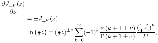
16: 10.15 Derivatives with Respect to Order

… ►

10.15.1 $$\frac{\partial J_{\pm \nu }\left(z\right)}{\partial \nu }=\pm J_{\pm \nu }\left(z\right)\ln \left(\frac{1}{2}z\right)\mp {(\frac{1}{2}z)}^{\pm \nu }\sum _{k=0}^{\mathrm{\infty }}{(-1)}^k\frac{\psi \left(k+1\pm \nu \right)}{\mathrm{\Gamma }\left(k+1\pm \nu \right)}\frac{{(\frac{1}{4}{z}^2)}^k}{k!},$$

ⓘ

Symbols:

$J_{\nu }\left(z\right)$: Bessel function of the first kind, $\mathrm{\Gamma }\left(z\right)$: gamma function, $\psi \left(z\right)$: psi (or digamma) function, $!$: factorial (as in $n!$), $\ln z$: principal branch of logarithm function, $\frac{\partial f}{\partial x}$: partial derivative of $f$ with respect to $x$ , $\partial x$: partial differential of $x$ , $k$: nonnegative integer, $z$: complex variable and $\nu$: complex parameter

A&S Ref:

9.1.64

Referenced by:

§10.15, §10.38, Erratum (V1.0.17) for Equations (10.15.1), (10.38.1)

Permalink:

http://dlmf.nist.gov/10.15.E1

Encodings:

pMML, png, TeX

Addition (effective with 1.0.17):

This equation has been generalized to include the additional case of $\partial J_{-\nu }\left(z\right)/\partial \nu$ because it will help the user who wants to combine it with (10.15.2).

See also:

Annotations for §10.15, §10.15 and Ch.10

…

17: 18.34 Bessel Polynomials

… ►

§18.34(i) Definitions and Recurrence Relation

►For the confluent hypergeometric function ${}_1{}^{}F_1^{}$ and the generalized hypergeometric function ${}_2{}^{}F_0^{}$, the Laguerre polynomial $L_n^{(\alpha )}$ and the Whittaker function $W_{\kappa ,\mu }$ see §16.2(ii), §16.2(iv), (18.5.12), and (13.14.3), respectively. … ►Hence the full system of polynomials $y_n(x;a)$ cannot be orthogonal on the line with respect to a positive weight function, but this is possible for a finite system of such polynomials, the Romanovski–Bessel polynomials, if : …The full system satisfies orthogonality with respect to a (not positive definite) moment functional; see Evans et al. (1993, (2.7)) for the simple expression of the moments ${\mu }_n$. … ►where primes denote derivatives with respect to $x$. …

18: 10.1 Special Notation

… ► ►►►►

$m,n$	integers. In §§10.47–10.71 $n$ is nonnegative.
…
$\mathit{\vartheta }$	$z(d/dz)$.
…
primes	derivatives with respect to argument, except where indicated otherwise.

… ►For the Kelvin functions the order $\nu$ is always assumed to be real. … ►Abramowitz and Stegun (1964): $j_n(z)$, $y_n(z)$, $h_n^{(1)}(z)$, $h_n^{(2)}(z)$, for ${𝗃}_n\left(z\right)$, ${𝗒}_n\left(z\right)$, ${𝗁}_n^{(1)}\left(z\right)$, ${𝗁}_n^{(2)}\left(z\right)$, respectively, when $n\ge 0$. ►Jeffreys and Jeffreys (1956): ${\mathrm{Hs}}_{\nu }(z)$ for $H_{\nu }^{(1)}\left(z\right)$, ${\mathrm{Hi}}_{\nu }(z)$ for $H_{\nu }^{(2)}\left(z\right)$, ${\mathrm{Kh}}_{\nu }(z)$ for $(2/\pi )K_{\nu }\left(z\right)$. …

19: 2.8 Differential Equations with a Parameter

… ►

2.8.1 $$d^{2}w/{dz}^2=\left(u^{2}f(z)+g(z)\right)w,$$

ⓘ

Symbols:

$\frac{df}{dx}$: derivative of $f$ with respect to $x$ , $f(x)$: function, $g(x)$: function, $w$: solution and $u$: large real or complex parameter

Referenced by:

§2.8(i), §2.8(v)

Permalink:

http://dlmf.nist.gov/2.8.E1

Encodings:

pMML, png, TeX

See also:

Annotations for §2.8(i), §2.8 and Ch.2

… ►

2.8.2 $$W={\dot{z}}^{-1/2}w,$$

ⓘ

Symbols:

$w$: solution, $W$: change of variable and $\dot{z}$: derivative of $z$ with respect to $\xi$

Permalink:

http://dlmf.nist.gov/2.8.E2

Encodings:

pMML, png, TeX

See also:

Annotations for §2.8(i), §2.8 and Ch.2

… ►

2.8.4 $$\psi (\xi )={\dot{z}}^{2}g(z)+{\dot{z}}^{1/2}\frac{d^2}{{d\xi }^2}({\dot{z}}^{-1/2}).$$

ⓘ

Symbols:

$\frac{df}{dx}$: derivative of $f$ with respect to $x$ , $g(x)$: function, $\dot{z}$: derivative of $z$ with respect to $\xi$ and $\psi (\xi )$: function

Permalink:

http://dlmf.nist.gov/2.8.E4

Encodings:

pMML, png, TeX

See also:

Annotations for §2.8(i), §2.8 and Ch.2

… ►

2.8.8 $$d^{2}W/{d\xi }^2=\left(u^2{\xi }^m+\psi (\xi )\right)W,$$

ⓘ

Symbols:

$\frac{df}{dx}$: derivative of $f$ with respect to $x$ , $u$: large real or complex parameter, $W$: change of variable and $\psi (\xi )$: function

Referenced by:

§2.8(i), §2.8(iv)

Permalink:

http://dlmf.nist.gov/2.8.E8

Encodings:

pMML, png, TeX

See also:

Annotations for §2.8(i), §2.8 and Ch.2

… ►

2.8.10 $$d^{2}W/{d\xi }^2=(u^2+\psi (\xi ))W,$$

ⓘ

Symbols:

$\frac{df}{dx}$: derivative of $f$ with respect to $x$ , $W_{n,j}(u,\xi )$: solution, $u$: large real or complex parameter and $\psi (\xi )$: function

Permalink:

http://dlmf.nist.gov/2.8.E10

Encodings:

pMML, png, TeX

See also:

Annotations for §2.8(ii), §2.8 and Ch.2

…

20: 4.24 Inverse Trigonometric Functions: Further Properties

… ►

4.24.7 $$\frac{d}{dz}\arcsin z={(1-z^2)}^{-1/2},$$

ⓘ

Symbols:

$\frac{df}{dx}$: derivative of $f$ with respect to $x$ , $\arcsin z$: arcsine function and $z$: complex variable

A&S Ref:

4.4.52

Permalink:

http://dlmf.nist.gov/4.24.E7

Encodings:

pMML, png, TeX

See also:

Annotations for §4.24(ii), §4.24 and Ch.4

►

4.24.8 $$\frac{d}{dz}\arccos z=-{(1-z^2)}^{-1/2},$$

ⓘ

Symbols:

$\frac{df}{dx}$: derivative of $f$ with respect to $x$ , $\arccos z$: arccosine function and $z$: complex variable

A&S Ref:

4.4.53

Permalink:

http://dlmf.nist.gov/4.24.E8

Encodings:

pMML, png, TeX

See also:

Annotations for §4.24(ii), §4.24 and Ch.4

… ►

4.24.10 $$\frac{d}{dz}\mathrm{arccsc}z=\mp \frac{1}{z{(z^2-1)}^{1/2}},$$ $\mathrm{\Re }z\gtrless 0$.

ⓘ

Symbols:

$\frac{df}{dx}$: derivative of $f$ with respect to $x$ , $\mathrm{arccsc}z$: arccosecant function, $\mathrm{\Re }$: real part and $z$: complex variable

A&S Ref:

4.4.57 (has an error.)

Referenced by:

§4.24(ii)

Permalink:

http://dlmf.nist.gov/4.24.E10

Encodings:

pMML, png, TeX

See also:

Annotations for §4.24(ii), §4.24 and Ch.4

►

4.24.11 $$\frac{d}{dz}\mathrm{arcsec}z=\pm \frac{1}{z{(z^2-1)}^{1/2}},$$ $\mathrm{\Re }z\gtrless 0$.

ⓘ

Symbols:

$\frac{df}{dx}$: derivative of $f$ with respect to $x$ , $\mathrm{arcsec}z$: arcsecant function, $\mathrm{\Re }$: real part and $z$: complex variable

A&S Ref:

4.4.56 (has an error.)

Referenced by:

§4.24(ii)

Permalink:

http://dlmf.nist.gov/4.24.E11

Encodings:

pMML, png, TeX

See also:

Annotations for §4.24(ii), §4.24 and Ch.4

…