variable%20boundaries

SearchAdvancedHelp

(0.001 seconds)

21—30 of 682 matching pages

21: 1.13 Differential Equations

… ►

§1.13(iv) Change of Variables

… ►

Elimination of First Derivative by Change of Independent Variable

… ►Assuming that $u(x)$ satisfies un-mixed boundary conditions of the form …or periodic boundary conditions … ►For a regular Sturm-Liouville system, equations (1.13.26) and (1.13.29) have: (i) identical eigenvalues, $\lambda$; (ii) the corresponding (real) eigenfunctions, $u(x)$ and $w(t)$, have the same number of zeros, also called nodes, for $t\in (0,c)$ as for $x\in (a,b)$; (iii) the eigenfunctions also satisfy the same type of boundary conditions, un-mixed or periodic, for both forms at the corresponding boundary points. …

22: 25.12 Polylogarithms

… ►

25.12.1 $${\mathrm{Li}}_2\left(z\right)\equiv \sum _{n=1}^{\mathrm{\infty }}\frac{z^n}{n^2},$$ $|z|\le 1$.

ⓘ

Defines:

${\mathrm{Li}}_2\left(z\right)$: dilogarithm

Symbols:

$\equiv$: equals by definition, $n$: nonnegative integer, $x$: real variable and $z$: complex variable

Keywords:

definition

Source:

Maximon (2003, (3.1), p. 2808)

A&S Ref:

27.7.2 (with $z=1-x$)

Referenced by:

§25.12(i), §25.12(i)

Permalink:

http://dlmf.nist.gov/25.12.E1

Encodings:

pMML, png, TeX

See also:

Annotations for §25.12(i), §25.12 and Ch.25

… ►

►►

Figure 25.12.1: Dilogarithm function ${\mathrm{Li}}_2\left(x\right)$, Magnify

►

►

►

Figure 25.12.2: Absolute value of the dilogarithm function $\left|{\mathrm{Li}}_2\left(x+\mathrm{i}y\right)\right|$, $-20\le x\le 20$, $-20\le y\le 20$. … Magnify 3D Help

… ►

25.12.10 $${\mathrm{Li}}_s\left(z\right)=\sum _{n=1}^{\mathrm{\infty }}\frac{z^n}{n^s}.$$

ⓘ

Defines:

${\mathrm{Li}}_s\left(z\right)$: polylogarithm

Symbols:

$n$: nonnegative integer, $s$: complex variable and $z$: complex variable

Keywords:

definition, infinite series, series representation

Source:

Lewin (1981, p. 236)

Referenced by:

(25.14.3)

Permalink:

http://dlmf.nist.gov/25.12.E10

Encodings:

pMML, png, TeX

See also:

Annotations for §25.12(ii), §25.12 and Ch.25

… ►

25.12.11 $${\mathrm{Li}}_s\left(z\right)\equiv \frac{z}{\mathrm{\Gamma }\left(s\right)}{\int }_0^{\mathrm{\infty }}\frac{x^{s-1}}{{\mathrm{e}}^x-z}dx,$$

ⓘ

Symbols:

$\mathrm{\Gamma }\left(z\right)$: gamma function, $dx$: differential of $x$ , $\equiv$: equals by definition, $\mathrm{e}$: base of natural logarithm, $\int$: integral, ${\mathrm{Li}}_s\left(z\right)$: polylogarithm, $x$: real variable, $s$: complex variable and $z$: complex variable

Keywords:

improper integral, integral representation

Source:

Lewin (1981, (7.188), p. 236)

Referenced by:

(25.12.16), §25.12(ii)

Permalink:

http://dlmf.nist.gov/25.12.E11

Encodings:

pMML, png, TeX

See also:

Annotations for §25.12(ii), §25.12(ii), §25.12 and Ch.25

…

23: 18.39 Applications in the Physical Sciences

… ►The solutions of (18.39.8) are subject to boundary conditions at $a$ and $b$. … ►The solutions (18.39.8) are called the stationary states as separation of variables in (18.39.9) yields solutions of form … ►Namely the $k$th eigenfunction, listed in order of increasing eigenvalues, starting at $k=0$, has precisely $k$ nodes, as real zeros of wave-functions away from boundaries are often referred to. … ►

§18.39(ii) A 3D Separable Quantum System, the Hydrogen Atom

… ►Derivations of (18.39.42) appear in Bethe and Salpeter (1957, pp. 12–20), and Pauling and Wilson (1985, Chapter V and Appendix VII), where the derivations are based on (18.39.36), and is also the notation of Piela (2014, §4.7), typifying the common use of the associated Coulomb–Laguerre polynomials in theoretical quantum chemistry. …

24: 1.18 Linear Second Order Differential Operators and Eigenfunction Expansions

… ►Ignoring the boundary value terms it follows that … ►Other choices of boundary conditions, identical for $f(x)$ and $g(x)$, and which also lead to the vanishing of the boundary terms in (1.18.26), each lead to a distinct self adjoint extension of $T$. … ►

Self-adjoint extensions of (1.18.28) and the Weyl alternative

… ►Boundary values and boundary conditions for the end point $b$ are defined in a similar way. If $n_1=1$ then there are no nonzero boundary values at $a$; if $n_1=2$ then the above boundary values at $a$ form a two-dimensional class. …

25: 25.3 Graphics

… ►

►►

Figure 25.3.1: Riemann zeta function $\zeta \left(x\right)$ and its derivative ${\zeta }^{\prime }\left(x\right)$, $-20\le x\le 10$. Magnify

…

26: 16.25 Methods of Computation

… ►Instead a boundary-value problem needs to be formulated and solved. …

27: 10.3 Graphics

… ►

§10.3(i) Real Order and Variable

… ►

§10.3(ii) Real Order, Complex Variable

… ►

►

►

Figure 10.3.14: $H_5^{(1)}\left(x+\mathrm{i}y\right)$, $-20\le x\le 10$, $-4\le y\le 4$. … Magnify 3D Help

… ►

►

►

Figure 10.3.16: $H_{5.5}^{(1)}\left(x+\mathrm{i}y\right)$, $-20\le x\le 10$, $-4\le y\le 4$. … Magnify 3D Help

►

§10.3(iii) Imaginary Order, Real Variable

…

28: 28.10 Integral Equations

… ►

28.10.1 $$\frac{2}{\pi }{\int }_0^{\pi /2}\cos \left(2h\cos z\cos t\right){\mathrm{ce}}_{2n}(t,h^2)dt=\frac{A_0^{2n}(h^2)}{{\mathrm{ce}}_{2n}(\frac{1}{2}\pi ,h^2)}{\mathrm{ce}}_{2n}(z,h^2),$$

ⓘ

Symbols:

${\mathrm{ce}}_n(z,q)$: Mathieu function, $\pi$: the ratio of the circumference of a circle to its diameter, $\cos z$: cosine function, $dx$: differential of $x$ , $\int$: integral, $h$: parameter, $n$: integer, $z$: complex variable and $A_m(q)$: Fourier coefficient

A&S Ref:

20.7.20 (in different form)

Permalink:

http://dlmf.nist.gov/28.10.E1

Encodings:

pMML, png, TeX

See also:

Annotations for §28.10(i), §28.10 and Ch.28

►

28.10.2 $$\frac{2}{\pi }{\int }_0^{\pi /2}\cosh \left(2h\sin z\sin t\right){\mathrm{ce}}_{2n}(t,h^2)dt=\frac{A_0^{2n}(h^2)}{{\mathrm{ce}}_{2n}(0,h^2)}{\mathrm{ce}}_{2n}(z,h^2),$$

ⓘ

Symbols:

${\mathrm{ce}}_n(z,q)$: Mathieu function, $\pi$: the ratio of the circumference of a circle to its diameter, $dx$: differential of $x$ , $\cosh z$: hyperbolic cosine function, $\int$: integral, $\sin z$: sine function, $h$: parameter, $n$: integer, $z$: complex variable and $A_m(q)$: Fourier coefficient

A&S Ref:

20.7.21 (in different form)

Permalink:

http://dlmf.nist.gov/28.10.E2

Encodings:

pMML, png, TeX

See also:

Annotations for §28.10(i), §28.10 and Ch.28

►

28.10.3 $$\frac{2}{\pi }{\int }_0^{\pi /2}\sin \left(2h\cos z\cos t\right){\mathrm{ce}}_{2n+1}(t,h^2)dt=-\frac{h{A}_1^{2n+1}(h^2)}{{\mathrm{ce}}_{2n+1}^{\prime }(\frac{1}{2}\pi ,h^2)}{\mathrm{ce}}_{2n+1}(z,h^2),$$

ⓘ

Symbols:

${\mathrm{ce}}_n(z,q)$: Mathieu function, $\pi$: the ratio of the circumference of a circle to its diameter, $\cos z$: cosine function, $dx$: differential of $x$ , $\int$: integral, $\sin z$: sine function, $h$: parameter, $n$: integer, $z$: complex variable and $A_m(q)$: Fourier coefficient

A&S Ref:

20.7.20 (in different form)

Permalink:

http://dlmf.nist.gov/28.10.E3

Encodings:

pMML, png, TeX

See also:

Annotations for §28.10(i), §28.10 and Ch.28

… ►

§28.10(iii) Further Equations

… ►For relations with variable boundaries see Volkmer (1983).

29: 9.18 Tables

… ►

§9.18(ii) Real Variables

… ►

Zhang and Jin (1996, p. 337) tabulates $\mathrm{Ai}\left(x\right)$, ${\mathrm{Ai}}^{\prime }\left(x\right)$, $\mathrm{Bi}\left(x\right)$, ${\mathrm{Bi}}^{\prime }\left(x\right)$ for $x=0(1)20$ to 8S and for $x=-20(1)0$ to 9D.

… ►

§9.18(iii) Complex Variables

… ►

Miller (1946) tabulates $a_k$, ${\mathrm{Ai}}^{\prime }\left(a_k\right)$, $a_k^{\prime }$, $\mathrm{Ai}\left(a_k^{\prime }\right)$, $k=1(1)50$; $b_k$, ${\mathrm{Bi}}^{\prime }\left(b_k\right)$, $b_k^{\prime }$, $\mathrm{Bi}\left(b_k^{\prime }\right)$, $k=1(1)20$. Precision is 8D. Entries for $k=1(1)20$ are reproduced in Abramowitz and Stegun (1964, Chapter 10).

►

Sherry (1959) tabulates $a_k$, ${\mathrm{Ai}}^{\prime }\left(a_k\right)$, $a_k^{\prime }$, $\mathrm{Ai}\left(a_k^{\prime }\right)$, $k=1(1)50$; 20S.

…

30: 28.32 Mathematical Applications

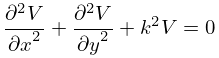
… ►If the boundary conditions in a physical problem relate to the perimeter of an ellipse, then elliptical coordinates are convenient. These are given by … ►

28.32.2 $$\frac{{\partial }^{2}V}{{\partial x}^2}+\frac{{\partial }^{2}V}{{\partial y}^2}+k^{2}V=0$$

ⓘ

Symbols:

$\frac{\partial f}{\partial x}$: partial derivative of $f$ with respect to $x$ , $\partial x$: partial differential of $x$ , $x$: real variable, $y$: real variable, $k$: parameter and $V(\xi ,\eta )$: solution

Referenced by:

§28.33(ii)

Permalink:

http://dlmf.nist.gov/28.32.E2

Encodings:

pMML, png, TeX

See also:

Annotations for §28.32(i), §28.32 and Ch.28

… ►This leads to integral equations and an integral relation between the solutions of Mathieu’s equation (setting $\zeta =\mathrm{i}\xi$, $z=\eta$ in (28.32.3)). … ►

28.32.6 $$w(z)={\int }_{ℒ}K(z,\zeta )u(\zeta )d\zeta$$

ⓘ

Symbols:

$dx$: differential of $x$ , $\int$: integral, $z$: complex variable, $\zeta$: variable, $u(\zeta )$: solution, $K(z,\zeta )$: solution and $ℒ$: curve

Permalink:

http://dlmf.nist.gov/28.32.E6

Encodings:

pMML, png, TeX

See also:

Annotations for §28.32(i), §28.32 and Ch.28

…