values at infinity

SearchAdvancedHelp

(0.006 seconds)

51—60 of 132 matching pages

51: 5.12 Beta Function

… ►In this section all fractional powers have their principal values, except where noted otherwise. … ►

5.12.3 $${\int }_0^{\mathrm{\infty }}\frac{t^{a-1}dt}{{(1+t)}^{a+b}}=\mathrm{B}(a,b).$$

ⓘ

Symbols:

$\mathrm{B}(a,b)$: beta function, $dx$: differential of $x$ , $\int$: integral, $a$: real or complex variable and $b$: real or complex variable

A&S Ref:

6.2.1 and 6.2.2

Referenced by:

§5.12

Permalink:

http://dlmf.nist.gov/5.12.E3

Encodings:

pMML, png, TeX

See also:

Annotations for §5.12, §5.12 and Ch.5

… ►

5.12.8 $$\frac{1}{2\pi }{\int }_{-\mathrm{\infty }}^{\mathrm{\infty }}\frac{dt}{{(w+\mathrm{i}t)}^a{(z-\mathrm{i}t)}^b}=\frac{{(w+z)}^{1-a-b}}{(a+b-1)\mathrm{B}(a,b)},$$ $\mathrm{\Re }\left(a+b\right)>1$, $\mathrm{\Re }w>0$, $\mathrm{\Re }z>0$.

ⓘ

Symbols:

$\mathrm{B}(a,b)$: beta function, $\pi$: the ratio of the circumference of a circle to its diameter, $dx$: differential of $x$ , $\mathrm{i}$: imaginary unit, $\int$: integral, $\mathrm{\Re }$: real part, $w$: real or complex variable, $z$: complex variable, $a$: real or complex variable and $b$: real or complex variable

Referenced by:

§5.12, §5.12

Permalink:

http://dlmf.nist.gov/5.12.E8

Encodings:

pMML, png, TeX

See also:

Annotations for §5.12, §5.12 and Ch.5

►In (5.12.8) the fractional powers have their principal values when $w>0$ and $z>0$, and are continued via continuity. … ►In (5.12.11) and (5.12.12) the fractional powers are continuous on the integration paths and take their principal values at the beginning. …

52: 11.13 Methods of Computation

… ►Although the power-series expansions (11.2.1) and (11.2.2), and the Bessel-function expansions of §11.4(iv) converge for all finite values of $z$, they are cumbersome to use when $|z|$ is large owing to slowness of convergence and cancellation. … ►For numerical purposes the most convenient of the representations given in §11.5, at least for real variables, include the integrals (11.5.2)–(11.5.5) for ${𝐊}_{\nu }\left(z\right)$ and ${𝐌}_{\nu }\left(z\right)$. … ►To insure stability the integration path must be chosen so that as we proceed along it the wanted solution grows in magnitude at least as rapidly as the complementary solutions. … ►For ${𝐌}_{\nu }\left(x\right)$ both forward and backward integration are unstable, and boundary-value methods are required (§3.7(iii)). … ►In consequence forward recurrence, backward recurrence, or boundary-value methods may be necessary. …

53: 14.22 Graphics

… ►In the graphics shown in this section, height corresponds to the absolute value of the function and color to the phase. … ►

►

►

Figure 14.22.1: $P_{1/2}^0\left(x+\mathrm{i}y\right)$, $-5\le x\le 5$, $-5\le y\le 5$. There is a cut along the real axis from $-\mathrm{\infty }$ to $-1$. Magnify 3D Help

►

►

►

Figure 14.22.2: $P_{1/2}^{-1/2}\left(x+\mathrm{i}y\right)$, $-5\le x\le 5$, $-5\le y\le 5$. There is a cut along the real axis from $-\mathrm{\infty }$ to $1$. Magnify 3D Help

►

►

►

Figure 14.22.3: $P_{1/2}^{-1}\left(x+\mathrm{i}y\right)$, $-5\le x\le 5$, $-5\le y\le 5$. There is a cut along the real axis from $-\mathrm{\infty }$ to $1$. Magnify 3D Help

…

54: 16.17 Definition

… ►

$L$ goes from $-\mathrm{i}\mathrm{\infty }$ to $\mathrm{i}\mathrm{\infty }$. The integral converges if and .

►

$L$ is a loop that starts at infinity on a line parallel to the positive real axis, encircles the poles of the $\mathrm{\Gamma }\left(b_{\mathrm{\ell }}-s\right)$ once in the negative sense and returns to infinity on another line parallel to the positive real axis. The integral converges for all $z$ ($\ne 0$) if , and for if $p=q\ge 1$.

►

$L$ is a loop that starts at infinity on a line parallel to the negative real axis, encircles the poles of the $\mathrm{\Gamma }\left(1-a_{\mathrm{\ell }}+s\right)$ once in the positive sense and returns to infinity on another line parallel to the negative real axis. The integral converges for all $z$ if $p>q$, and for $|z|>1$ if $p=q\ge 1$.

… ►When more than one of Cases (i), (ii), and (iii) is applicable the same value is obtained for the Meijer $G$-function. …

55: 14.21 Definitions and Basic Properties

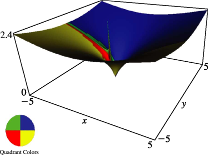
… ► $P_{\nu }^{\pm \mu }\left(z\right)$ and ${𝑸}_{\nu }^{\mu }\left(z\right)$ exist for all values of $\nu$, $\mu$, and $z$, except possibly $z=\pm 1$ and $\mathrm{\infty }$, which are branch points (or poles) of the functions, in general. When $z$ is complex $P_{\nu }^{\pm \mu }\left(z\right)$, $Q_{\nu }^{\mu }\left(z\right)$, and ${𝑸}_{\nu }^{\mu }\left(z\right)$ are defined by (14.3.6)–(14.3.10) with $x$ replaced by $z$: the principal branches are obtained by taking the principal values of all the multivalued functions appearing in these representations when $z\in (1,\mathrm{\infty })$, and by continuity elsewhere in the $z$-plane with a cut along the interval $(-\mathrm{\infty },1]$; compare §4.2(i). … … ►

§14.21(iii) Properties

… ►This includes, for example, the Wronskian relations (14.2.7)–(14.2.11); hypergeometric representations (14.3.6)–(14.3.10) and (14.3.15)–(14.3.20); results for integer orders (14.6.3)–(14.6.5), (14.6.7), (14.6.8), (14.7.6), (14.7.7), and (14.7.11)–(14.7.16); behavior at singularities (14.8.7)–(14.8.16); connection formulas (14.9.11)–(14.9.16); recurrence relations (14.10.3)–(14.10.7). …

56: 2.4 Contour Integrals

… ►as $z\to \mathrm{\infty }$ in the sector $|\mathrm{ph}z|\le \frac{1}{2}\pi -\delta$ (), with $z^{(s+\lambda )/\mu }$ assigned its principal value. … ►is seen to converge absolutely at each limit, and be independent of $\sigma \in [c,\mathrm{\infty })$. … ►If this integral converges uniformly at each limit for all sufficiently large $t$, then by the Riemann–Lebesgue lemma (§1.8(i)) … ►Cases in which $p^{\prime }(t_0)\ne 0$ are usually handled by deforming the integration path in such a way that the minimum of $\mathrm{\Re }\left(zp(t)\right)$ is attained at a saddle point or at an endpoint. … ►with $p,q$ and their derivatives evaluated at $t_0$. …

57: 25.2 Definition and Expansions

… ►

25.2.1 $$\zeta \left(s\right)=\sum _{n=1}^{\mathrm{\infty }}\frac{1}{n^s}.$$

ⓘ

Defines:

$\zeta \left(s\right)$: Riemann zeta function

Symbols:

$n$: nonnegative integer and $s$: complex variable

Keywords:

definition, infinite series

Sources:

Apostol (1976, Chapter 12); Riemann (1859, p. 136)

A&S Ref:

23.2.1

Referenced by:

(25.11.2), (25.2.2), (25.2.4), §25.2(ii), Erratum (V1.0.17) for Equation (25.2.4)

Permalink:

http://dlmf.nist.gov/25.2.E1

Encodings:

pMML, png, TeX

See also:

Annotations for §25.2(i), §25.2 and Ch.25

… ►It is a meromorphic function whose only singularity in $ℂ$ is a simple pole at $s=1$, with residue 1. … ►

25.2.2 $$\zeta \left(s\right)=\frac{1}{1-2^{-s}}\sum _{n=0}^{\mathrm{\infty }}\frac{1}{{(2n+1)}^s},$$ $\mathrm{\Re }s>1$.

ⓘ

Symbols:

$\zeta \left(s\right)$: Riemann zeta function, $\mathrm{\Re }$: real part, $n$: nonnegative integer and $s$: complex variable

Keywords:

infinite series

Proof sketch:

Derivable from (25.2.1).

A&S Ref:

23.2.20 (is the special case with integer values of $s$)

Referenced by:

(25.11.11)

Permalink:

http://dlmf.nist.gov/25.2.E2

Encodings:

pMML, png, TeX

See also:

Annotations for §25.2(ii), §25.2 and Ch.25

►

25.2.3 $$\zeta \left(s\right)=\frac{1}{1-2^{1-s}}\sum _{n=1}^{\mathrm{\infty }}\frac{{(-1)}^{n-1}}{n^s},$$ $\mathrm{\Re }s>0$.

ⓘ

Symbols:

$\zeta \left(s\right)$: Riemann zeta function, $\mathrm{\Re }$: real part, $n$: nonnegative integer and $s$: complex variable

Keywords:

infinite series

Source:

Apostol (1976, (27), p. 292)

A&S Ref:

23.2.19 (is the special case with integer values of $s$)

Referenced by:

§25.11(x)

Permalink:

http://dlmf.nist.gov/25.2.E3

Encodings:

pMML, png, TeX

See also:

Annotations for §25.2(ii), §25.2 and Ch.25

►

25.2.4 $$\zeta \left(s\right)=\frac{1}{s-1}+\sum _{n=0}^{\mathrm{\infty }}\frac{{(-1)}^n}{n!}{\gamma }_n{(s-1)}^n,$$

ⓘ

Symbols:

$\zeta \left(s\right)$: Riemann zeta function, ${\gamma }_n$: Stieltjes constants, $!$: factorial (as in $n!$), $\mathrm{\Re }$: real part, $n$: nonnegative integer and $s$: complex variable

Keywords:

infinite series, Laurent series

Sources:

Hardy (1912, p. 216); mistakenly missing factor of ${(-1)}^n/n!$; Ivić (1985, (1.11), p. 4)

A&S Ref:

23.2.5 (with unnecessary constraint removed)

Referenced by:

Erratum (V1.0.17) for Equation (25.2.4), Erratum (V1.0.23) for Subsection 25.2(ii) Other Infinite Series

Permalink:

http://dlmf.nist.gov/25.2.E4

Encodings:

pMML, png, TeX

Clarification (effective with 1.0.17):

Originally this equation had the constraint $\mathrm{\Re }s>0$. This constraint is unnecessary because, as stated after (25.2.1), $\zeta \left(s\right)$ is meromorphic with a simple pole at $s=1$.

Suggested 2017-12-05 by John Harper

See also:

Annotations for §25.2(ii), §25.2 and Ch.25

…

58: 28.2 Definitions and Basic Properties

… ►This equation has regular singularities at 0 and 1, both with exponents 0 and $\frac{1}{2}$, and an irregular singular point at $\mathrm{\infty }$. … ►Furthermore, a solution $w$ with given initial constant values of $w$ and $w^{\prime }$ at a point $z_0$ is an entire function of the three variables $z$, $a$, and $q$. … ►For nonnegative real values of $q$, see Figure 28.2.1. … ►

Distribution

… ►

Change of Sign of $q$

…

59: 5.2 Definitions

… ►

5.2.1 $$\mathrm{\Gamma }\left(z\right)={\int }_0^{\mathrm{\infty }}{\mathrm{e}}^{-t}{t}^{z-1}dt,$$ $\mathrm{\Re }z>0$.

ⓘ

Defines:

$\mathrm{\Gamma }\left(z\right)$: gamma function

Symbols:

$dx$: differential of $x$ , $\mathrm{e}$: base of natural logarithm, $\int$: integral, $\mathrm{\Re }$: real part and $z$: complex variable

A&S Ref:

6.1.1

Referenced by:

§10.43(iii), (25.11.27), (25.11.28), (25.5.6), (25.5.7), §5.9(i), §5.9(ii), §8.21(ii), (9.12.17)

Permalink:

http://dlmf.nist.gov/5.2.E1

Encodings:

pMML, png, TeX

See also:

Annotations for §5.2(i), §5.2(i), §5.2 and Ch.5

… ►It is a meromorphic function with no zeros, and with simple poles of residue ${(-1)}^n/n!$ at $z=-n$. $1/\mathrm{\Gamma }\left(z\right)$ is entire, with simple zeros at $z=-n$. …$\psi \left(z\right)$ is meromorphic with simple poles of residue $-1$ at $z=-n$. … ►

5.2.3 $$\gamma =\underset{n\to \mathrm{\infty }}{lim}\left(1+\frac{1}{2}+\frac{1}{3}+\mathrm{\cdots }+\frac{1}{n}-\ln n\right)=\mathrm{0.57721\hspace{0.33em}56649\hspace{0.33em}01532\hspace{0.33em}86060}\mathrm{\dots }.$$

ⓘ

Defines:

$\gamma$: Euler’s constant

Symbols:

$\ln z$: principal branch of logarithm function and $n$: nonnegative integer

A&S Ref:

6.1.3 (where the 10D value is given, and Table 1.1 where the 24D value is given.)

Notes:

For more digits see OEIS Sequence A001620; see also Sloane (2003).

Referenced by:

§4.4(iii)

Permalink:

http://dlmf.nist.gov/5.2.E3

Encodings:

pMML, png, TeX

See also:

Annotations for §5.2(ii), §5.2 and Ch.5

…

60: 1.18 Linear Second Order Differential Operators and Eigenfunction Expansions

… ►For this latter see Simon (1973), and Reinhardt (1982); wherein advantage is taken of the fact that although branch points are actual singularities of an analytic function, the location of the branch cuts are often at our disposal, as they are not singularities of the function, but simply arbitrary lines to keep a function single valued, and thus only singularities of a specific representation of that analytic function. … ►Suppose that $X$ is the whole real line in one dimension, and that $q(x)$, in (1.18.28) has (non-oscillatory) limits of $0$ at both $\pm \mathrm{\infty }$, and thus a continuous spectrum on $𝝈\ge 0$. … ►In unusual cases $N=\mathrm{\infty }$, even for all $\mathrm{\ell }$, such as in the case of the Schrödinger–Coulomb problem ($V=-r^{-1}$) discussed in §18.39 and §33.14, where the point spectrum actually accumulates at the onset of the continuum at $\lambda =0$, implying an essential singularity, as well as a branch point, in matrix elements of the resolvent, (1.18.66). … ►If $n_1=1$ then there are no nonzero boundary values at $a$; if $n_1=2$ then the above boundary values at $a$ form a two-dimensional class. Similarly at $b$. …