values at infinity

SearchAdvancedHelp

(0.007 seconds)

31—40 of 132 matching pages

31: 9.19 Approximations

… ►

Martín et al. (1992) provides two simple formulas for approximating $\mathrm{Ai}\left(x\right)$ to graphical accuracy, one for , the other for .

►

Moshier (1989, §6.14) provides minimax rational approximations for calculating $\mathrm{Ai}\left(x\right)$, ${\mathrm{Ai}}^{\prime }\left(x\right)$, $\mathrm{Bi}\left(x\right)$, ${\mathrm{Bi}}^{\prime }\left(x\right)$. They are in terms of the variable $\zeta$, where $\zeta =\frac{2}{3}{x}^{3/2}$ when $x$ is positive, $\zeta =\frac{2}{3}{(-x)}^{3/2}$ when $x$ is negative, and $\zeta =0$ when $x=0$. The approximations apply when , that is, when or . The precision in the coefficients is 21S.

… ►These expansions are for real arguments $x$ and are supplied in sets of four for each function, corresponding to intervals , $a\le x\le 0$, $0\le x\le b$, . … ►

Corless et al. (1992) describe a method of approximation based on subdividing $ℂ$ into a triangular mesh, with values of $\mathrm{Ai}\left(z\right)$, ${\mathrm{Ai}}^{\prime }\left(z\right)$ stored at the nodes. $\mathrm{Ai}\left(z\right)$ and ${\mathrm{Ai}}^{\prime }\left(z\right)$ are then computed from Taylor-series expansions centered at one of the nearest nodes. The Taylor coefficients are generated by recursion, starting from the stored values of $\mathrm{Ai}\left(z\right)$, ${\mathrm{Ai}}^{\prime }\left(z\right)$ at the node. Similarly for $\mathrm{Bi}\left(z\right)$, ${\mathrm{Bi}}^{\prime }\left(z\right)$.

… ►

MacLeod (1994) supplies Chebyshev-series expansions to cover $\mathrm{Gi}\left(x\right)$ for and $\mathrm{Hi}\left(x\right)$ for . The Chebyshev coefficients are given to 20D.

32: 14.16 Zeros

… ►For uniform asymptotic approximations for the zeros of ${𝖯}_n^{-m}\left(x\right)$ in the interval when $n\to \mathrm{\infty }$ with $m$ $(\ge 0)$ fixed, see Olver (1997b, p. 469). ►

§14.16(iii) Interval

► $P_{\nu }^{\mu }\left(x\right)$ has exactly one zero in the interval $(1,\mathrm{\infty })$ if either of the following sets of conditions holds: … ►For all other values of $\mu$ and $\nu$ (with $\nu \ge -\frac{1}{2}$) $P_{\nu }^{\mu }\left(x\right)$ has no zeros in the interval $(1,\mathrm{\infty })$. ► ${𝑸}_{\nu }^{\mu }\left(x\right)$ has no zeros in the interval $(1,\mathrm{\infty })$ when $\nu >-1$, and at most one zero in the interval $(1,\mathrm{\infty })$ when .

33: 4.2 Definitions

… ►This is a multivalued function of $z$ with branch point at $z=0$. … ► $\ln z$ is a single-valued analytic function on $ℂ\setminus (-\mathrm{\infty },0]$ and real-valued when $z$ ranges over the positive real numbers. … ► … ►The principal value is …This is an analytic function of $z$ on $ℂ\setminus (-\mathrm{\infty },0]$, and is two-valued and discontinuous on the cut shown in Figure 4.2.1, unless $a\in \mathbb{Z}$. …

34: 4.3 Graphics

… ►Figure 4.3.2 illustrates the conformal mapping of the strip onto the whole $w$-plane cut along the negative real axis, where $w={\mathrm{e}}^z$ and $z=\ln w$ (principal value). …Lines parallel to the real axis in the $z$-plane map onto rays in the $w$-plane, and lines parallel to the imaginary axis in the $z$-plane map onto circles centered at the origin in the $w$-plane. In the labeling of corresponding points $r$ is a real parameter that can lie anywhere in the interval $(0,\mathrm{\infty })$. … ►In the graphics shown in this subsection height corresponds to the absolute value of the function and color to the phase. … ►

►

►

Figure 4.3.3: $\ln \left(x+\mathrm{i}y\right)$ (principal value). … Magnify 3D Help

…

35: 22.5 Special Values

§22.5 Special Values

►

§22.5(i) Special Values of $z$

►Table 22.5.1 gives the value of each of the 12 Jacobian elliptic functions, together with its $z$-derivative (or at a pole, the residue), for values of $z$ that are integer multiples of $K$, $\mathrm{i}{K}^{\prime }$. … ►Table 22.5.2 gives $\mathrm{sn}(z,k)$, $\mathrm{cn}(z,k)$, $\mathrm{dn}(z,k)$ for other special values of $z$. … ►

§22.5(ii) Limiting Values of $k$

…

36: 4.37 Inverse Hyperbolic Functions

… ►

§4.37(i) General Definitions

… ►In (4.37.2) the integration path may not pass through either of the points $\pm 1$, and the function ${(t^2-1)}^{1/2}$ assumes its principal value when $t\in (1,\mathrm{\infty })$. … ►

§4.37(ii) Principal Values

… ►Compare the principal value of the logarithm (§4.2(i)). … ►Throughout this subsection all quantities assume their principal values. …

37: 2.11 Remainder Terms; Stokes Phenomenon

… ►If the results agree within $S$ significant figures, then it is likely—but not certain—that the truncated asymptotic series will yield at least $S$ correct significant figures for larger values of $x$. … ►In this way we arrive at hyperasymptotic expansions. … ►17408, compared with the correct value … ►17045, which is much closer to the true value. … ►Comparison with the true value …

38: 18.30 Associated OP’s

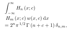
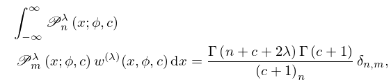
… ►These constraints guarantee that the orthogonality only involves the integral $x\in [0,\mathrm{\infty })$, as above. ►For other cases there may also be, in addition to a possible integral as in (18.30.10), a finite sum of discrete weights on the negative real $x$-axis each multiplied by the polynomial product evaluated at the corresponding values of $x$, as in (18.2.3). … ►

18.30.14 $${\int }_{-\mathrm{\infty }}^{\mathrm{\infty }}{H}_n(x;c)H_m(x;c)w(x,c)dx=2^n{\pi }^{1/2}\mathrm{\Gamma }\left(n+c+1\right){\delta }_{n,m},$$ $c>-1$,

ⓘ

Symbols:

$\mathrm{\Gamma }\left(z\right)$: gamma function, ${\delta }_{j,k}$: Kronecker delta, $H_n(x;c)$: associated Hermite polynomial, $\pi$: the ratio of the circumference of a circle to its diameter, $dx$: differential of $x$ , $\int$: integral, $w(x)$: weight function, $m$: nonnegative integer, $n$: nonnegative integer and $x$: real variable

Permalink:

http://dlmf.nist.gov/18.30.E14

Encodings:

pMML, png, TeX

See also:

Annotations for §18.30(iv), §18.30 and Ch.18

… ►

18.30.17 $${\int }_{-\mathrm{\infty }}^{\mathrm{\infty }}{𝒫}_n^{\lambda }(x;\varphi ,c){𝒫}_m^{\lambda }(x;\varphi ,c)w^{(\lambda )}(x,\varphi ,c)dx=\frac{\mathrm{\Gamma }\left(n+c+2\lambda \right)\mathrm{\Gamma }\left(c+1\right)}{{\left(c+1\right)}_n}{\delta }_{n,m},$$ or ,

ⓘ

Symbols:

$\mathrm{\Gamma }\left(z\right)$: gamma function, ${\delta }_{j,k}$: Kronecker delta, ${\left(a\right)}_n$: Pochhammer’s symbol (or shifted factorial), ${𝒫}_n^{\lambda }(x;\varphi ,c)$: associated Meixner–Pollaczek polynomial, $\pi$: the ratio of the circumference of a circle to its diameter, $dx$: differential of $x$ , $\int$: integral, $w(x)$: weight function, $m$: nonnegative integer, $n$: nonnegative integer and $x$: real variable

Sources:

Askey and Wimp (1984, (1.9)); Pollaczek (1950, formula following (16))

Permalink:

http://dlmf.nist.gov/18.30.E17

Encodings:

pMML, png, TeX

See also:

Annotations for §18.30(v), §18.30 and Ch.18

… ►

18.30.25 $$\underset{n\to \mathrm{\infty }}{lim}{F}_n(x)=\underset{n\to \mathrm{\infty }}{lim}{p}_n^{(0)}(z)/p_n(z)=\frac{1}{{\mu }_0}{\int }_a^b\frac{d\mu (x)}{z-x},$$ $z\in ℂ\backslash [a,b]$.

ⓘ

Symbols:

$[a,b]$: closed interval, $ℂ$: complex plane, $dx$: differential of $x$ , $\in$: element of, $\int$: integral, $p_n(x)$: polynomial of degree $n$ , $z$: complex variable, $n$: nonnegative integer and $x$: real variable

Proved:

Chihara (1978, Chapter III, Theorem 4.3)(proved)

Referenced by:

§18.30(vi), §18.30(vii)

Permalink:

http://dlmf.nist.gov/18.30.E25

Encodings:

pMML, png, TeX

See also:

Annotations for §18.30(vi), §18.30(vi), §18.30 and Ch.18

…

39: 2.3 Integrals of a Real Variable

… ►Assume that $q(t)$ again has the expansion (2.3.7) and this expansion is infinitely differentiable, $q(t)$ is infinitely differentiable on $(0,\mathrm{\infty })$, and each of the integrals $\int {\mathrm{e}}^{\mathrm{i}xt}{q}^{(s)}(t)dt$, $s=0,1,2,\mathrm{\dots }$, converges at $t=\mathrm{\infty }$, uniformly for all sufficiently large $x$. … ►Assume also that ${\partial }^{2}p(\alpha ,t)/{\partial t}^2$ and $q(\alpha ,t)$ are continuous in $\alpha$ and $t$, and for each $\alpha$ the minimum value of $p(\alpha ,t)$ in $[0,k)$ is at $t=\alpha$, at which point $\partial p(\alpha ,t)/\partial t$ vanishes, but both ${\partial }^{2}p(\alpha ,t)/{\partial t}^2$ and $q(\alpha ,t)$ are nonzero. When $x\to +\mathrm{\infty }$ Laplace’s method (§2.3(iii)) applies, but the form of the resulting approximation is discontinuous at $\alpha =0$. … ► $\kappa =\kappa (\alpha )$ being the value of $w$ at $t=k$. We now expand $f(\alpha ,w)$ in a Taylor series centered at the peak value $w=a$ of the exponential factor in the integrand: …

40: 19.3 Graphics

… ►

►

►

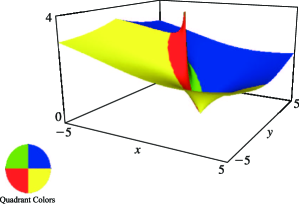
Figure 19.3.4: $E(\varphi ,k)$ as a function of $k^2$ and ${\sin }^2\varphi$ for $-1\le k^2\le 2$, $0\le {\sin }^2\varphi \le 1$. If ${\sin }^2\varphi =1$ ($\ge k^2$), then the function reduces to $E\left(k\right)$, with value 1 at $k^2=1$. … Magnify 3D Help

… ►

►

►

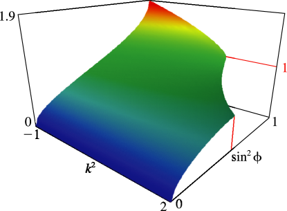
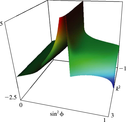
Figure 19.3.6: $\mathrm{\Pi }(\varphi ,2,k)$ as a function of $k^2$ and ${\sin }^2\varphi$ for $-1\le k^2\le 3$, . …If ${\sin }^2\varphi =1$ ($>k^2$), then the function reduces to $\mathrm{\Pi }(2,k)$ with Cauchy principal value $K\left(k\right)-\mathrm{\Pi }(\frac{1}{2}{k}^2,k)$, which tends to $-\mathrm{\infty }$ as $k^2\to 1-$. …Its value tends to $-\mathrm{\infty }$ as $k^2\to 1+$ by (19.6.6), and to the negative of the second lemniscate constant (see (19.20.22)) as $k^2(={\csc }^2\varphi )\to 2-$. Magnify 3D Help

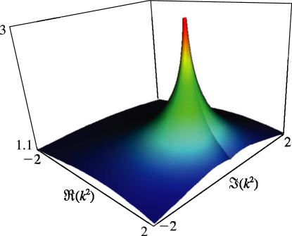
… ►In Figures 19.3.7 and 19.3.8 for complete Legendre’s elliptic integrals with complex arguments, height corresponds to the absolute value of the function and color to the phase. … ►

►

►

Figure 19.3.9: $\mathrm{\Re }\left(K\left(k\right)\right)$ as a function of complex $k^2$ for $-2\le \mathrm{\Re }\left(k^2\right)\le 2$, $-2\le \mathrm{\Im }\left(k^2\right)\le 2$. …On the branch cut ($k^2\ge 1$) it is infinite at $k^2=1$, and has the value $K(1/k)/k$ when $k^2>1$. Magnify 3D Help

…