sine%20and%20cosine%20integrals

(0.004 seconds)

11—14 of 14 matching pages

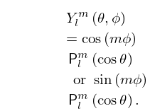
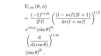
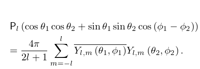
11: 14.30 Spherical and Spheroidal Harmonics

… ►

14.30.2

Y_{l}^{m}\left(\theta,\phi\right)=\cos\left(m\phi\right)\mathsf{P}^{m}_{l}% \left(\cos\theta\right)\text{ or }\sin\left(m\phi\right)\mathsf{P}^{m}_{l}% \left(\cos\theta\right).

ⓘ

Defines:: $Y_{\NVar{l}}^{\NVar{m}}\left(\NVar{\theta},\NVar{\phi}\right)$ : surface harmonic of the first kind
Symbols:: $\mathsf{P}^{\NVar{\mu}}_{\NVar{\nu}}\left(\NVar{x}\right)$ : Ferrers function of the first kind, $\cos\NVar{z}$ : cosine function, $\sin\NVar{z}$ : sine function, $m$ : integer and $l$ : nonnegative integer
Referenced by:: §14.30(i), Erratum (V1.0.25) for Section 14.30
Permalink:: http://dlmf.nist.gov/14.30.E2
Encodings:: pMML, png, TeX
See also:: Annotations for §14.30(i), §14.30 and Ch.14

… ►

14.30.3

Y_{{l},{m}}\left(\theta,\phi\right)=\frac{(-1)^{l+m}}{2^{l}l!}\left(\frac{(l-m% )!(2l+1)}{4\pi(l+m)!}\right)^{1/2}e^{im\phi}\left(\sin\theta\right)^{m}\*\left% (\frac{\mathrm{d}}{\mathrm{d}(\cos\theta)}\right)^{l+m}\left(\sin\theta\right)% ^{2l}.

ⓘ

Symbols:: $\pi$ : the ratio of the circumference of a circle to its diameter, $\cos\NVar{z}$ : cosine function, $\frac{\mathrm{d}\NVar{f}}{\mathrm{d}\NVar{x}}$ : derivative of $f$ with respect to $x$ , $\mathrm{e}$ : base of natural logarithm, $!$ : factorial (as in $n!$ ), $\mathrm{i}$ : imaginary unit, $\sin\NVar{z}$ : sine function, $Y_{{\NVar{l}},{\NVar{m}}}\left(\NVar{\theta},\NVar{\phi}\right)$ : spherical harmonic, $m$ : integer and $l$ : nonnegative integer
Referenced by:: §14.30(ii)
Permalink:: http://dlmf.nist.gov/14.30.E3
Encodings:: pMML, png, TeX
See also:: Annotations for §14.30(ii), §14.30(ii), §14.30 and Ch.14

… ►See also (34.3.22), and for further related integrals see Askey et al. (1986). … ►where

\mathbf{a}=\left(\tfrac{1}{2\lambda}-\tfrac{\lambda}{2},-\tfrac{\mathrm{i}}{2% \lambda}-\tfrac{\mathrm{i}\lambda}{2},1\right)

and

\mathbf{x}=\left(r\sin\theta\cos\phi,r\sin\theta\sin\phi,r\cos\theta\right)

. … ►

14.30.9

\mathsf{P}_{l}\left(\cos\theta_{1}\cos\theta_{2}+\sin\theta_{1}\sin\theta_{2}% \cos\left(\phi_{1}-\phi_{2}\right)\right)=\frac{4\pi}{2l+1}\sum_{m=-l}^{l}% \overline{Y_{{l},{m}}\left(\theta_{1},\phi_{1}\right)}Y_{{l},{m}}\left(\theta_% {2},\phi_{2}\right).

ⓘ

Symbols:: $\pi$ : the ratio of the circumference of a circle to its diameter, $\overline{\NVar{z}}$ : complex conjugate, $\cos\NVar{z}$ : cosine function, $\mathsf{P}_{\NVar{\nu}}\left(\NVar{x}\right)=\mathsf{P}^{0}_{\nu}\left(x\right)$ : Ferrers function of the first kind, $\sin\NVar{z}$ : sine function, $Y_{{\NVar{l}},{\NVar{m}}}\left(\NVar{\theta},\NVar{\phi}\right)$ : spherical harmonic, $m$ : integer and $l$ : nonnegative integer
Referenced by:: §18.18(ii)
Permalink:: http://dlmf.nist.gov/14.30.E9
Encodings:: pMML, png, TeX
Notational Change (effective with 1.0.19):: As a notational clarification, the first spherical harmonic in the sum over $m$ has been explicity marked up as a complex conjugate.
See also:: Annotations for §14.30(iii), §14.30(iii), §14.30 and Ch.14

…

	Open Source	With Book	Commercial
…
6 Exponential, Logarithmic, Sine, and Cosine Integrals
6.21(ii) $E_{1}\left(x\right)$ , $\operatorname{Ei}\left(x\right)$ , $\operatorname{Si}\left(x\right)$ , $\operatorname{Ci}\left(x\right)$ , $\operatorname{Shi}\left(x\right)$ , $\operatorname{Chi}\left(x\right)$ , $x\in\mathbb{R}$	✓	✓	✓	✓	✓	✓	✓	✓	✓	✓	✓	✓	✓	✓	✓	✓	✓	✓	✓	✓	✓	✓
6.21(iii) $E_{1}\left(z\right)$ , $\operatorname{Si}\left(z\right)$ , $\operatorname{Ci}\left(z\right)$ , $\operatorname{Shi}\left(z\right)$ , $\operatorname{Chi}\left(z\right)$ , $z\in\mathbb{C}$	✓	✓				✓		✓		✓	✓	✓							✓	✓	✓
…
7.25(iv) $C\left(x\right)$ , $S\left(x\right)$ , $\mathrm{f}\left(x\right)$ , $\mathrm{g}\left(x\right)$ , $x\in\mathbb{R}$	✓		✓					✓		a	✓	✓	✓	✓	✓	✓	✓	✓	✓	✓	✓
7.25(v) $C\left(z\right)$ , $S\left(z\right)$ , $z\in\mathbb{C}$	✓									a	✓								✓	✓	✓
…

13: Errata

… ►

Subsection 19.11(i)

A sentence and unnumbered equation

R_{C}\left(\gamma-\delta,\gamma\right)=\frac{-1}{\sqrt{\delta}}\operatorname{% arctan}\left(\frac{\sqrt{\delta}\sin\theta\sin\phi\sin\psi}{\alpha^{2}-1-% \alpha^{2}\cos\theta\cos\phi\cos\psi}\right),

were added which indicate that care must be taken with the multivalued functions in (19.11.5). See (Cayley, 1961, pp. 103-106).

Suggested by Albert Groenenboom.

… ►

Equation (10.22.72)

10.22.72

\int_{0}^{\infty}J_{\mu}\left(at\right)J_{\nu}\left(bt\right)J_{\nu}\left(ct% \right)t^{1-\mu}\,\mathrm{d}t=\frac{(bc)^{\mu-1}\sin\left((\mu-\nu)\pi\right)(% \sinh\chi)^{\mu-\frac{1}{2}}}{(\frac{1}{2}{\pi}^{3})^{\frac{1}{2}}a^{\mu}}{% \mathrm{e}}^{(\mu-\frac{1}{2})\mathrm{i}\pi}Q^{\frac{1}{2}-\mu}_{\nu-\frac{1}{% 2}}\left(\cosh\chi\right),

\Re\mu>-\tfrac{1}{2},\Re\nu>-1,a>b+c,\cosh\chi=(a^{2}-b^{2}-c^{2})/(2bc)

Originally, the factor on the right-hand side was written as $\frac{(bc)^{\mu-1}\cos\left(\nu\pi\right)(\sinh\chi)^{\mu-\frac{1}{2}}}{(\frac% {1}{2}{\pi}^{3})^{\frac{1}{2}}a^{\mu}}$ , which was taken directly from Watson (1944, p. 412, (13.46.5)), who uses a different normalization for the associated Legendre function of the second kind $Q^{\mu}_{\nu}$ . Watson’s $Q_{\nu}^{\mu}$ equals $\frac{\sin\left((\nu+\mu)\pi\right)}{\sin\left(\nu\pi\right)}{\mathrm{e}}^{-% \mu\pi\mathrm{i}}Q^{\mu}_{\nu}$ in the DLMF.

Reported by Arun Ravishankar on 2018-10-22

… ►

Section 1.14

There have been extensive changes in the notation used for the integral transforms defined in §1.14. These changes are applied throughout the DLMF. The following table summarizes the changes.

Transform	New	Abbreviated	Old
	Notation	Notation	Notation
Fourier	$\mathscr{F}\left(f\right)\left(x\right)$	$\mathscr{F}\mskip-3.0muf\mskip 3.0mu\left(x\right)$
Fourier Cosine	$\mathscr{F}_{\mkern-3.0muc}\left(f\right)\left(x\right)$	$\mathscr{F}_{\mkern-3.0muc}\mskip-1.0muf\mskip 3.0mu\left(x\right)$
Fourier Sine	$\mathscr{F}_{\mkern-2.0mus}\left(f\right)\left(x\right)$	$\mathscr{F}_{\mkern-2.0mus}\mskip-1.0muf\mskip 3.0mu\left(x\right)$
Laplace	$\mathscr{L}\left(f\right)\left(s\right)$	$\mathscr{L}\mskip-3.0muf\mskip 3.0mu\left(s\right)$	$\mathscr{L}(f(t);s)$
Mellin	$\mathscr{M}\left(f\right)\left(s\right)$	$\mathscr{M}\mskip-3.0muf\mskip 3.0mu\left(s\right)$	$\mathscr{M}(f;s)$
Hilbert	$\mathcal{H}\left(f\right)\left(s\right)$	$\mathcal{H}\mskip-3.0muf\mskip 3.0mu\left(s\right)$	$\mathcal{H}(f;s)$
Stieltjes	$\mathcal{S}\left(f\right)\left(s\right)$	$\mathcal{S}\mskip-3.0muf\mskip 3.0mu\left(s\right)$	$\mathcal{S}(f;s)$

Previously, for the Fourier, Fourier cosine and Fourier sine transforms, either temporary local notations were used or the Fourier integrals were written out explicitly.

… ►

Equation (4.21.1)

4.21.1

\sin u\pm\cos u=\sqrt{2}\sin\left(u\pm\tfrac{1}{4}\pi\right)=\pm\sqrt{2}\cos% \left(u\mp\tfrac{1}{4}\pi\right)

Originally the symbol $\pm$ was missing after the second equal sign.

Reported 2012-09-27 by Dennis Heim.

… ►

Chapters 8, 20, 36

Several new equations have been added. See (8.17.24), (20.7.34), §20.11(v), (26.12.27), (36.2.28), and (36.2.29).

…

14: 3.4 Differentiation

… ►If

f

can be extended analytically into the complex plane, then from Cauchy’s integral formula (§1.9(iii)) …The integral on the right-hand side can be approximated by the composite trapezoidal rule (3.5.2). … ►The integral (3.4.18) becomes …With the choice

r=k

(which is crucial when

k

is large because of numerical cancellation) the integrand equals

e^{k}

at the dominant points

\theta=0,2\pi

, and in combination with the factor

k^{-k}

in front of the integral sign this gives a rough approximation to

1/k!

. …As explained in §§3.5(i) and 3.5(ix) the composite trapezoidal rule can be very efficient for computing integrals with analytic periodic integrands. …

sine%20and%20cosine%20integrals

11—14 of 14 matching pages

11: 14.30 Spherical and Spheroidal Harmonics

12: Software Index

13: Errata

14: 3.4 Differentiation