roots of constants

SearchAdvancedHelp

(0.002 seconds)

11—20 of 42 matching pages

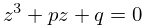
11: 4.43 Cubic Equations

… ►Let $p(\ne 0)$ and $q$ be real constants and …The roots of ►

4.43.2 $$z^3+pz+q=0$$

ⓘ

Symbols:

$\pi$: the ratio of the circumference of a circle to its diameter, $\cosh z$: hyperbolic cosine function, $\sinh z$: hyperbolic sine function, $\mathrm{i}$: imaginary unit, $\sin z$: sine function, $a$: real or complex constant, $z$: complex variable, $p$: real constant and $q$: real constant

Referenced by:

(4.43.1), §4.43

Permalink:

http://dlmf.nist.gov/4.43.E2

Encodings:

pMML, png, TeX

Errata (effective with 1.0.10):

Cases (a), (b), and (c) of of this equation have been corrected. Formerly, with constants $C$ and $D$ given in Eq. (4.43.1), they read

1. $A\sin a$, $A\sin \left(a+\frac{2}{3}\pi \right)$, and $A\sin \left(a+\frac{4}{3}\pi \right)$, with $\sin \left(3a\right)=C$, when and $C\le 1$.

2. $A\cosh a$, $A\cosh \left(a+\frac{2}{3}\pi \mathrm{i}\right)$, and $A\cosh \left(a+\frac{4}{3}\pi \mathrm{i}\right)$, with $\cosh \left(3a\right)=C$, when and $C>1$.

3. $B\sinh a$, $B\sinh \left(a+\frac{2}{3}\pi \mathrm{i}\right)$, and $B\sinh \left(a+\frac{4}{3}\pi \mathrm{i}\right)$, with $\sinh \left(3a\right)=D$, when $p>0$.

Reported 2014-10-31 by Masataka Urago

See also:

Annotations for §4.43 and Ch.4

… ►Note that in Case (a) all the roots are real, whereas in Cases (b) and (c) there is one real root and a conjugate pair of complex roots. …

12: 4.30 Elementary Properties

… ►

Table 4.30.1: Hyperbolic functions: interrelations. All square roots have their principal values when the functions are real, nonnegative, and finite.

► ►►

	$\sinh \theta =a$	$\cosh \theta =a$	$\tanh \theta =a$	$\mathrm{csch}\theta =a$	$\mathrm{sech}\theta =a$	$\coth \theta =a$
…

►

13: 4.16 Elementary Properties

… ►

Table 4.16.3: Trigonometric functions: interrelations. All square roots have their principal values when the functions are real, nonnegative, and finite.

► ►►

	$\sin \theta =a$	$\cos \theta =a$	$\tan \theta =a$	$\csc \theta =a$	$\sec \theta =a$	$\cot \theta =a$
…

►

14: 18.39 Applications in the Physical Sciences

… ►All are written in the same form as the product of three factors: the square root of a weight function $w(x)$, the corresponding OP or EOP, and constant factors ensuring unit normalization. …

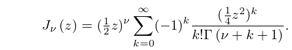
15: 10.2 Definitions

… ►

10.2.2 $$J_{\nu }\left(z\right)={(\frac{1}{2}z)}^{\nu }\sum _{k=0}^{\mathrm{\infty }}{(-1)}^k\frac{{(\frac{1}{4}{z}^2)}^k}{k!\mathrm{\Gamma }\left(\nu +k+1\right)}.$$

ⓘ

Defines:

$J_{\nu }\left(z\right)$: Bessel function of the first kind

Symbols:

$\mathrm{\Gamma }\left(z\right)$: gamma function, $!$: factorial (as in $n!$), $k$: nonnegative integer, $z$: complex variable and $\nu$: complex parameter

A&S Ref:

9.1.10

Referenced by:

§10.11, §10.16, §10.19(i), §10.22(ii), §10.22(iii), §10.24, §10.53, §10.65(i), §10.7(i), §10.74(ii), §10.8, §18.38(iii), §8.6(i)

Permalink:

http://dlmf.nist.gov/10.2.E2

Encodings:

pMML, png, TeX

See also:

Annotations for §10.2(ii), §10.2(ii), §10.2 and Ch.10

… ►as $z\to \mathrm{\infty }$ in $-2\pi +\delta \le \mathrm{ph}z\le \pi -\delta$, where $\delta$ is an arbitrary small positive constant. …The principal branches correspond to principal values of the square roots in (10.2.5) and (10.2.6), again with a cut in the $z$-plane along the interval $(-\mathrm{\infty },0]$. …

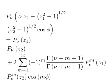
16: 14.28 Sums

… ►

14.28.1 $$P_{\nu }\left(z_1{z}_2-{\left(z_1^2-1\right)}^{1/2}{\left(z_2^2-1\right)}^{1/2}\cos \varphi \right)=P_{\nu }\left(z_1\right)P_{\nu }\left(z_2\right)+2\sum _{m=1}^{\mathrm{\infty }}{(-1)}^m\frac{\mathrm{\Gamma }\left(\nu -m+1\right)}{\mathrm{\Gamma }\left(\nu +m+1\right)}{P}_{\nu }^m\left(z_1\right)P_{\nu }^m(z_2)\cos \left(m\varphi \right),$$

ⓘ

Symbols:

$\mathrm{\Gamma }\left(z\right)$: gamma function, $P_{\nu }^{\mu }\left(z\right)$: associated Legendre function of the first kind, $\cos z$: cosine function, $P_{\nu }\left(z\right)=P_{\nu }^0\left(z\right)$: Legendre function of the first kind, $z$: complex variable, $m$: nonnegative integer and $\nu$: general degree

Permalink:

http://dlmf.nist.gov/14.28.E1

Encodings:

pMML, png, TeX

See also:

Annotations for §14.28(i), §14.28 and Ch.14

►where the branches of the square roots have their principal values when $z_1,z_2\in (1,\mathrm{\infty })$ and are continuous when $z_1,z_2\in ℂ\setminus (0,1]$. …

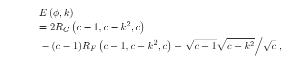
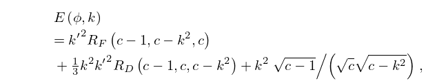
17: 19.25 Relations to Other Functions

… ►

19.25.7 $$E(\varphi ,k)=2R_G(c-1,c-k^2,c)-(c-1)R_F(c-1,c-k^2,c)-\sqrt{c-1}\sqrt{c-k^2}/\sqrt{c},$$

ⓘ

Symbols:

$R_F(x,y,z)$: symmetric elliptic integral of first kind, $R_G(x,y,z)$: symmetric elliptic integral of second kind, $E(\varphi ,k)$: Legendre’s incomplete elliptic integral of the second kind, $\varphi$: real or complex argument and $k$: real or complex modulus

Referenced by:

§19.25(i), §19.25(i), §19.25(iii), Figure 19.3.4, Figure 19.3.4, Figure 19.3.4, §19.36(ii), Erratum (V1.1.3) for Chapter 19

Permalink:

http://dlmf.nist.gov/19.25.E7

Encodings:

pMML, png, TeX

Correction (effective with 1.1.3):

The factors inside the square root on the right-hand side were written as products to ensure the correct multivalued behavior.

Suggested 2021-06-07 by Luc Maisonobe

See also:

Annotations for §19.25(i), §19.25 and Ch.19

… ►

19.25.10 $$E(\varphi ,k)=k_{}^{\prime }{}_{}{}^2{R}_F(c-1,c-k^2,c)+\frac{1}{3}{k}^{2}k_{}^{\prime }{}_{}{}^2{R}_D(c-1,c,c-k^2)+k^2\sqrt{c-1}/\left(\sqrt{c}\sqrt{c-k^2}\right),$$ $c>k^2$,

ⓘ

Symbols:

$R_D(x,y,z)$: elliptic integral symmetric in only two variables, $R_F(x,y,z)$: symmetric elliptic integral of first kind, $E(\varphi ,k)$: Legendre’s incomplete elliptic integral of the second kind, $\varphi$: real or complex argument, $k$: real or complex modulus and $k^{\prime }$: complementary modulus

Referenced by:

§19.25(i), §19.30(i), §19.36(i), §19.6(iv), Erratum (V1.1.3) for Chapter 19

Permalink:

http://dlmf.nist.gov/19.25.E10

Encodings:

pMML, png, TeX

Correction (effective with 1.1.3):

The factors inside the square root on the right-hand side were written as products to ensure the correct multivalued behavior.

Suggested 2021-06-07 by Luc Maisonobe

See also:

Annotations for §19.25(i), §19.25 and Ch.19

… ►

19.25.35 $$z+2\omega =\pm R_F(\mathrm{\wp }\left(z\right)-e_1,\mathrm{\wp }\left(z\right)-e_2,\mathrm{\wp }\left(z\right)-e_3),$$

ⓘ

Symbols:

$R_F(x,y,z)$: symmetric elliptic integral of first kind, $\mathrm{\wp }\left(z\right)$ (= $\mathrm{\wp }\left(z|𝕃\right)$ = $\mathrm{\wp }(z;g_2,g_3)$): Weierstrass $\mathrm{\wp }$-function, $e_j$: Weierstrass lattice roots and $z$: complex number

Proof sketch:

Use (23.6.36) with $z=\mathrm{\wp }\left(\omega \right)$ as prescribed in the text that follows (23.6.36), substitute $u=t+\mathrm{\wp }\left(\omega \right)$ and compare with (19.16.1). The undetermined $\pm$ is a consequence of the multivaluedness of the square-roots in (19.16.4).

Referenced by:

(19.25.38), (19.25.40), §19.25(v), §19.25(vi), §19.25(vi), §20.9(i), Erratum (V1.1.0) for Subsection 19.25(vi)

Permalink:

http://dlmf.nist.gov/19.25.E35

Encodings:

pMML, png, TeX

Correction (effective with 1.1.0):

This equation has been corrected, namely the left-hand side which was originally $z$, has been replaced by $z+2\omega$ and the right-hand side has been multiplied by $\pm 1$.

See also:

Annotations for §19.25(vi), §19.25 and Ch.19

… ►

19.25.36 $$\mathrm{\wp }\left(z\right)-e_j\in ℂ\setminus (-\mathrm{\infty },0],$$ $j=1,2,3.$

ⓘ

Symbols:

$\mathrm{\wp }\left(z\right)$ (= $\mathrm{\wp }\left(z|𝕃\right)$ = $\mathrm{\wp }(z;g_2,g_3)$): Weierstrass $\mathrm{\wp }$-function, $e_j$: Weierstrass lattice roots, $ℂ$: complex plane, $\in$: element of, $(a,b]$: half-closed interval, $\setminus$: set subtraction, $j$: $(=1,2,3)$ and $z$: complex number

Referenced by:

(19.25.39)

Permalink:

http://dlmf.nist.gov/19.25.E36

Encodings:

pMML, png, TeX

See also:

Annotations for §19.25(vi), §19.25 and Ch.19

… ►

19.25.38 $${\omega }_j=R_F(0,e_j-e_k,e_j-e_{\mathrm{\ell }}),$$

ⓘ

Symbols:

$R_F(x,y,z)$: symmetric elliptic integral of first kind, $e_j$: Weierstrass lattice roots, $j$: $(=1,2,3)$ , $z$: complex number, $k$: $(=1,2,3)$ , $\mathrm{\ell }$: $(=1,2,3)$ and ${\omega }_j$: nonzero complex number

Proof sketch:

Take $z=-\omega$ in (19.25.35).

Referenced by:

§19.25(vi), §19.25(vi)

Permalink:

http://dlmf.nist.gov/19.25.E38

Encodings:

pMML, png, TeX

See also:

Annotations for §19.25(vi), §19.25 and Ch.19

…

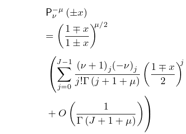
18: 14.15 Uniform Asymptotic Approximations

… ►

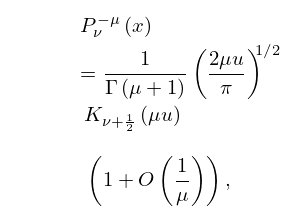
14.15.1 $${𝖯}_{\nu }^{-\mu }\left(\pm x\right)={\left(\frac{1\mp x}{1\pm x}\right)}^{\mu /2}\left(\sum _{j=0}^{J-1}\frac{{\left(\nu +1\right)}_j{\left(-\nu \right)}_j}{j!\mathrm{\Gamma }\left(j+1+\mu \right)}{\left(\frac{1\mp x}{2}\right)}^j+O\left(\frac{1}{\mathrm{\Gamma }\left(J+1+\mu \right)}\right)\right)$$

ⓘ

Symbols:

$O\left(x\right)$: order not exceeding, $\mathrm{\Gamma }\left(z\right)$: gamma function, : Ferrers function of the first kind, ${\left(a\right)}_n$: Pochhammer’s symbol (or shifted factorial), $!$: factorial (as in $n!$), $x$: real variable, $\mu$: general order, $\nu$: general degree and $J$: nonnegative integer

Referenced by:

§14.15(i)

Permalink:

http://dlmf.nist.gov/14.15.E1

Encodings:

pMML, png, TeX

See also:

Annotations for §14.15(i), §14.15 and Ch.14

… ►In other words, the convergent hypergeometric series expansions of ${𝖯}_{\nu }^{-\mu }\left(\pm x\right)$ are also generalized (and uniform) asymptotic expansions as $\mu \to \mathrm{\infty }$, with scale $1/\mathrm{\Gamma }\left(j+1+\mu \right)$, $j=0,1,2,\mathrm{\dots }$; compare §2.1(v). … ►

14.15.2 $$P_{\nu }^{-\mu }\left(x\right)=\frac{1}{\mathrm{\Gamma }\left(\mu +1\right)}{\left(\frac{2\mu u}{\pi }\right)}^{1/2}{K}_{\nu +\frac{1}{2}}\left(\mu u\right)\left(1+O\left(\frac{1}{\mu }\right)\right),$$

ⓘ

Symbols:

$O\left(x\right)$: order not exceeding, $\mathrm{\Gamma }\left(z\right)$: gamma function, $P_{\nu }^{\mu }\left(z\right)$: associated Legendre function of the first kind, $\pi$: the ratio of the circumference of a circle to its diameter, $K_{\nu }\left(z\right)$: modified Bessel function of the second kind, $x$: real variable, $\mu$: general order, $\nu$: general degree and $u$

Referenced by:

§14.15(i)

Permalink:

http://dlmf.nist.gov/14.15.E2

Encodings:

pMML, png, TeX

See also:

Annotations for §14.15(i), §14.15 and Ch.14

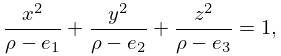
… ►In this and subsequent subsections $\delta$ denotes an arbitrary constant such that . … ►where $x=X_c$ denotes the largest positive root of the equation $U(-c,x)=\overline{U}(-c,x)$. …

19: 18.37 Classical OP’s in Two or More Variables

… ►where $c_j$ are real or complex constants, with $c_0\ne 0$; … ►

§18.37(iii) OP’s Associated with Root Systems

►Orthogonal polynomials associated with root systems are certain systems of trigonometric polynomials in several variables, symmetric under a certain finite group (Weyl group), and orthogonal on a torus. …In several variables they occur, for $q=1$, as Jack polynomials and also as Jacobi polynomials associated with root systems; see Macdonald (1995, Chapter VI, §10), Stanley (1989), Kuznetsov and Sahi (2006, Part 1), Heckman (1991). For general $q$ they occur as Macdonald polynomials for root system $A_n$ , as Macdonald polynomials for general root systems, and as Macdonald–Koornwinder polynomials; see Macdonald (1995, Chapter VI), Macdonald (2000, 2003), Koornwinder (1992).

20: 23.21 Physical Applications

… ►Ellipsoidal coordinates $(\xi ,\eta ,\zeta )$ may be defined as the three roots $\rho$ of the equation ►

23.21.1 $$\frac{x^2}{\rho -e_1}+\frac{y^2}{\rho -e_2}+\frac{z^2}{\rho -e_3}=1,$$

ⓘ

Symbols:

$e_j$: Weierstrass lattice roots, $𝕃$: lattice, $x$: real part of $z$ , $y$: imaginary part of $z$ , $z$: complex and $\rho$: roots

Permalink:

http://dlmf.nist.gov/23.21.E1

Encodings:

pMML, png, TeX

See also:

Annotations for §23.21(iii), §23.21 and Ch.23

►where $x,y,z$ are the corresponding Cartesian coordinates and $e_1$, $e_2$, $e_3$ are constants. … ►

23.21.3 $$f(\rho )=2{\left((\rho -e_1)(\rho -e_2)(\rho -e_3)\right)}^{1/2}.$$

ⓘ

Symbols:

$e_j$: Weierstrass lattice roots, $𝕃$: lattice, $\rho$: roots and $f(\rho )$: function

Permalink:

http://dlmf.nist.gov/23.21.E3

Encodings:

pMML, png, TeX

See also:

Annotations for §23.21(iii), §23.21 and Ch.23

►Another form is obtained by identifying $e_1$, $e_2$, $e_3$ as lattice roots (§23.3(i)), and setting …