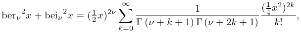
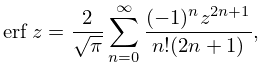
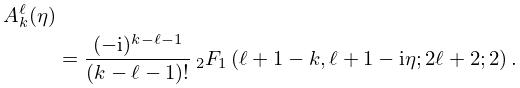
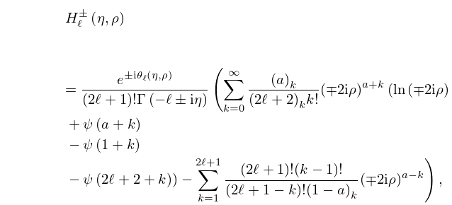
power-series%20expansions%20in%20q

SearchAdvancedHelp

(0.005 seconds)

11—20 of 948 matching pages

11: 14.32 Methods of Computation

… ►Essentially the same comments that are made in §15.19 concerning the computation of hypergeometric functions apply to the functions described in the present chapter. In particular, for small or moderate values of the parameters $\mu$ and $\nu$ the power-series expansions of the various hypergeometric function representations given in §§14.3(i)–14.3(iii), 14.19(ii), and 14.20(i) can be selected in such a way that convergence is stable, and reasonably rapid, especially when the argument of the functions is real. In other cases recurrence relations (§14.10) provide a powerful method when applied in a stable direction (§3.6); see Olver and Smith (1983) and Gautschi (1967). … ►

Application of the uniform asymptotic expansions for large values of the parameters given in §§14.15 and 14.20(vii)–14.20(ix).

… ►

Evaluation (§3.10) of the continued fractions given in §14.14. See Gil and Segura (2000).

…

12: 4.6 Power Series

§4.6 Power Series

►

§4.6(i) Logarithms

… ►

Binomial Expansion

►

4.6.7 $${(1+z)}^a=1+\frac{a}{1!}z+\frac{a(a-1)}{2!}{z}^2+\frac{a(a-1)(a-2)}{3!}{z}^3+\mathrm{\cdots },$$

ⓘ

Symbols:

$!$: factorial (as in $n!$), $a$: real or complex constant and $z$: complex variable

Referenced by:

§4.6(ii), §4.6(ii)

Permalink:

http://dlmf.nist.gov/4.6.E7

Encodings:

pMML, png, TeX

See also:

Annotations for §4.6(ii), §4.6(ii), §4.6 and Ch.4

… ►Note that (4.6.7) is a generalization of the binomial expansion (1.2.2) with the binomial coefficients defined in (1.2.6).

13: 10.65 Power Series

§10.65 Power Series

… ►

§10.65(iii) Cross-Products and Sums of Squares

►

10.65.6 $${\mathrm{ber}}_{\nu }^{2}x+{\mathrm{bei}}_{\nu }^{2}x={(\frac{1}{2}x)}^{2\nu }\sum _{k=0}^{\mathrm{\infty }}\frac{1}{\mathrm{\Gamma }\left(\nu +k+1\right)\mathrm{\Gamma }\left(\nu +2k+1\right)}\frac{{(\frac{1}{4}{x}^2)}^{2k}}{k!},$$

ⓘ

Symbols:

$\mathrm{\Gamma }\left(z\right)$: gamma function, ${\mathrm{bei}}_{\nu }\left(x\right)$: Kelvin function, ${\mathrm{ber}}_{\nu }\left(x\right)$: Kelvin function, $!$: factorial (as in $n!$), $k$: nonnegative integer, $x$: real variable and $\nu$: complex parameter

A&S Ref:

9.9.28

Permalink:

http://dlmf.nist.gov/10.65.E6

Encodings:

pMML, png, TeX

See also:

Annotations for §10.65(iii), §10.65 and Ch.10

… ►

§10.65(iv) Compendia

►For further power series summable in terms of Kelvin functions and their derivatives see Hansen (1975).

14: 28.6 Expansions for Small $q$

… ►

§28.6(i) Eigenvalues

►Leading terms of the power series for $a_m\left(q\right)$ and $b_m\left(q\right)$ for $m\le 6$ are: … ►Numerical values of the radii of convergence ${\rho }_n^{(j)}$ of the power series (28.6.1)–(28.6.14) for $n=0,1,\mathrm{\dots },9$ are given in Table 28.6.1. … ►

Table 28.6.1: Radii of convergence for power-series expansions of eigenvalues of Mathieu’s equation.

► ►►

$n$	${\rho }_n^{(1)}$		${\rho }_n^{(2)}$		${\rho }_n^{(3)}$
…

►

… ►

§28.6(ii) Functions ${\mathrm{ce}}_n$ and ${\mathrm{se}}_n$

…

15: 23.9 Laurent and Other Power Series

§23.9 Laurent and Other Power Series

… ►Explicit coefficients $c_n$ in terms of $c_2$ and $c_3$ are given up to $c_{19}$ in Abramowitz and Stegun (1964, p. 636). ►For $j=1,2,3$, and with $e_j$ as in §23.3(i), …Also, Abramowitz and Stegun (1964, (18.5.25)) supplies the first 22 terms in the reverted form of (23.9.2) as $1/\mathrm{\wp }\left(z\right)\to 0$. ►For $z\in ℂ$ …

16: 7.6 Series Expansions

§7.6 Series Expansions

►

§7.6(i) Power Series

►

7.6.1 $$\mathrm{erf}z=\frac{2}{\sqrt{\pi }}\sum _{n=0}^{\mathrm{\infty }}\frac{{(-1)}^n{z}^{2n+1}}{n!(2n+1)},$$

ⓘ

Symbols:

$\pi$: the ratio of the circumference of a circle to its diameter, $\mathrm{erf}z$: error function, $!$: factorial (as in $n!$), $z$: complex variable and $n$: nonnegative integer

A&S Ref:

7.1.5

Referenced by:

§7.6(i)

Permalink:

http://dlmf.nist.gov/7.6.E1

Encodings:

pMML, png, TeX

See also:

Annotations for §7.6(i), §7.6 and Ch.7

… ►The series in this subsection and in §7.6(ii) converge for all finite values of $|z|$. ►

§7.6(ii) Expansions in Series of Spherical Bessel Functions

…

17: 33.23 Methods of Computation

… ►The power-series expansions of §§33.6 and 33.19 converge for all finite values of the radii $\rho$ and $r$, respectively, and may be used to compute the regular and irregular solutions. … ►Thus the regular solutions can be computed from the power-series expansions (§§33.6, 33.19) for small values of the radii and then integrated in the direction of increasing values of the radii. On the other hand, the irregular solutions of §§33.2(iii) and 33.14(iii) need to be integrated in the direction of decreasing radii beginning, for example, with values obtained from asymptotic expansions (§§33.11 and 33.21). … ►Thompson and Barnett (1985, 1986) and Thompson (2004) use combinations of series, continued fractions, and Padé-accelerated asymptotic expansions (§3.11(iv)) for the analytic continuations of Coulomb functions. ►Noble (2004) obtains double-precision accuracy for $W_{-\eta ,\mu }\left(2\rho \right)$ for a wide range of parameters using a combination of recurrence techniques, power-series expansions, and numerical quadrature; compare (33.2.7). …

18: 33.6 Power-Series Expansions in $\rho$

§33.6 Power-Series Expansions in $\rho$

… ►or in terms of the hypergeometric function (§§15.1, 15.2(i)), ►

33.6.4 $$A_k^{\mathrm{\ell }}(\eta )=\frac{{(-\mathrm{i})}^{k-\mathrm{\ell }-1}}{(k-\mathrm{\ell }-1)!}{}_2{}^{}F_1^{}(\mathrm{\ell }+1-k,\mathrm{\ell }+1-\mathrm{i}\eta ;2\mathrm{\ell }+2;2).$$

ⓘ

Symbols:

${}_2{}^{}F_1^{}(a,b;c;z)$: $=F(a,b;c;z)$ notation for Gauss’ hypergeometric function, $!$: factorial (as in $n!$), $\mathrm{i}$: imaginary unit, $k$: nonnegative integer, $\mathrm{\ell }$: nonnegative integer, $\eta$: real parameter and $A_{\mathrm{\ell }+1}^{\mathrm{\ell }}$: coefficient

Referenced by:

§33.6

Permalink:

http://dlmf.nist.gov/33.6.E4

Encodings:

pMML, png, TeX

See also:

Annotations for §33.6 and Ch.33

►

33.6.5 $$H_{\mathrm{\ell }}^{\pm }(\eta ,\rho )=\frac{{\mathrm{e}}^{\pm \mathrm{i}{\theta }_{\mathrm{\ell }}(\eta ,\rho )}}{(2\mathrm{\ell }+1)!\mathrm{\Gamma }\left(-\mathrm{\ell }\pm \mathrm{i}\eta \right)}\left(\sum _{k=0}^{\mathrm{\infty }}\frac{{\left(a\right)}_k}{{\left(2\mathrm{\ell }+2\right)}_{k}k!}{(\mp 2\mathrm{i}\rho )}^{a+k}\left(\ln \left(\mp 2\mathrm{i}\rho \right)+\psi \left(a+k\right)-\psi \left(1+k\right)-\psi \left(2\mathrm{\ell }+2+k\right)\right)-\sum _{k=1}^{2\mathrm{\ell }+1}\frac{(2\mathrm{\ell }+1)!(k-1)!}{(2\mathrm{\ell }+1-k)!{\left(1-a\right)}_k}{(\mp 2\mathrm{i}\rho )}^{a-k}\right),$$

ⓘ

Symbols:

${\theta }_{\mathrm{\ell }}(\eta ,\rho )$: phase of Coulomb functions, $\mathrm{\Gamma }\left(z\right)$: gamma function, ${\left(a\right)}_n$: Pochhammer’s symbol (or shifted factorial), $\psi \left(z\right)$: psi (or digamma) function, $\mathrm{e}$: base of natural logarithm, $!$: factorial (as in $n!$), $\mathrm{i}$: imaginary unit, $H_{\mathrm{\ell }}^{\pm }(\eta ,\rho )$: irregular Coulomb radial functions, $\ln z$: principal branch of logarithm function, $k$: nonnegative integer, $\mathrm{\ell }$: nonnegative integer, $\rho$: nonnegative real variable, $\eta$: real parameter and $a$: variable

A&S Ref:

14.1.14 (equivalent)

Referenced by:

§33.13, §33.6, §33.6, Erratum (V1.0.19) for Equation (33.6.5)

Permalink:

http://dlmf.nist.gov/33.6.E5

Encodings:

pMML, png, TeX

Errata (effective with 1.0.19):

On the right-hand side the factor in the denominator was incorrectly written as $\mathrm{\Gamma }\left(-\mathrm{\ell }+\mathrm{i}\eta \right)$. This has been corrected to $\mathrm{\Gamma }\left(-\mathrm{\ell }\pm \mathrm{i}\eta \right)$.

Reported 2018-05-15 by Ian Thompson

See also:

Annotations for §33.6 and Ch.33

… ►Corresponding expansions for $H_{\mathrm{\ell }}^{\pm }{}_{}{}^{\prime }(\eta ,\rho )$ can be obtained by combining (33.6.5) with (33.4.3) or (33.4.4).

19: 33.19 Power-Series Expansions in $r$

§33.19 Power-Series Expansions in $r$

… ►

33.19.3 $$2\pi h(ϵ,\mathrm{\ell };r)=\sum _{k=0}^{2\mathrm{\ell }}\frac{(2\mathrm{\ell }-k)!{\gamma }_k}{k!}{(2r)}^{k-\mathrm{\ell }}-\sum _{k=0}^{\mathrm{\infty }}{\delta }_k{r}^{k+\mathrm{\ell }+1}-A(ϵ,\mathrm{\ell })\left(2\ln |2r/\kappa |+\mathrm{\Re }\psi \left(\mathrm{\ell }+1+\kappa \right)+\mathrm{\Re }\psi \left(-\mathrm{\ell }+\kappa \right)\right)f(ϵ,\mathrm{\ell };r),$$ $r\ne 0$.

ⓘ

Symbols:

$f(ϵ,\mathrm{\ell };r)$: regular Coulomb function, $h(ϵ,\mathrm{\ell };r)$: irregular Coulomb function, $\pi$: the ratio of the circumference of a circle to its diameter, $\psi \left(z\right)$: psi (or digamma) function, $!$: factorial (as in $n!$), $\ln z$: principal branch of logarithm function, $\mathrm{\Re }$: real part, $k$: nonnegative integer, $\mathrm{\ell }$: nonnegative integer, $r$: real variable, $ϵ$: real parameter, $\kappa$: quantity, $A(ϵ,\mathrm{\ell })$: function, ${\gamma }_k$: term and ${\delta }_k$: term

Referenced by:

§33.19

Permalink:

http://dlmf.nist.gov/33.19.E3

Encodings:

pMML, png, TeX

See also:

Annotations for §33.19 and Ch.33

… ►The expansions (33.19.1) and (33.19.3) converge for all finite values of $r$, except $r=0$ in the case of (33.19.3).

20: 3.10 Continued Fractions

… ►

§3.10(ii) Relations to Power Series

… ►

Stieltjes Fractions

… ►We say that it corresponds to the formal power series … ►For several special functions the $S$-fractions are known explicitly, but in any case the coefficients $a_n$ can always be calculated from the power-series coefficients by means of the quotient-difference algorithm; see Table 3.10.1. … ►We say that it is associated with the formal power series $f(z)$ in (3.10.7) if the expansion of its $n$th convergent $C_n$ in ascending powers of $z$, agrees with (3.10.7) up to and including the term in $z^{2n-1}$, $n=1,2,3,\mathrm{\dots }$. …