partial%20fractions
(0.001 seconds)
21—30 of 256 matching pages
21: 1.9 Calculus of a Complex Variable
…
►
►
…
►Conversely, if at a given point the partial derivatives , , , and exist, are continuous, and satisfy (1.9.25), then is differentiable at .
…
►
Bilinear Transformation
… ►Other names for the bilinear transformation are fractional linear transformation, homographic transformation, and Möbius transformation. …22: 21.7 Riemann Surfaces
23: 9.18 Tables
…
►
•
…
►
•
►
•
►
•
…
►
•
Zhang and Jin (1996, p. 337) tabulates , , , for to 8S and for to 9D.
Sherry (1959) tabulates , , , , ; 20S.
Zhang and Jin (1996, p. 339) tabulates , , , , , , , , ; 8D.
24: 22.12 Expansions in Other Trigonometric Series and Doubly-Infinite Partial Fractions: Eisenstein Series
§22.12 Expansions in Other Trigonometric Series and Doubly-Infinite Partial Fractions: Eisenstein Series
… ►
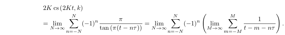
22.12.13
25: 33.23 Methods of Computation
…
►Cancellation errors increase with increases in and , and may be estimated by comparing the final sum of the series with the largest partial sum.
…
►
§33.23(v) Continued Fractions
►§33.8 supplies continued fractions for and . … ►Thompson and Barnett (1985, 1986) and Thompson (2004) use combinations of series, continued fractions, and Padé-accelerated asymptotic expansions (§3.11(iv)) for the analytic continuations of Coulomb functions. …26: 1.10 Functions of a Complex Variable
…
►Let be a bounded domain with boundary and let .
If is continuous on and analytic in , then attains its maximum on .
…
►The convergence of the infinite product is uniform if the sequence of partial products converges uniformly.
…
►
§1.10(x) Infinite Partial Fractions
… ►Mittag-Leffler’s Expansion
…27: 23.21 Physical Applications
…
►
§23.21(ii) Nonlinear Evolution Equations
►Airault et al. (1977) applies the function to an integrable classical many-body problem, and relates the solutions to nonlinear partial differential equations. … ►
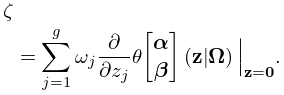
23.21.2
…
►
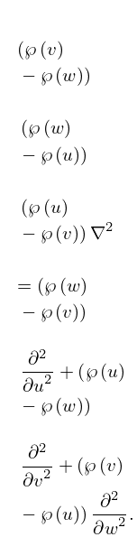
23.21.5
…
