of the path order

SearchAdvancedHelp

(0.002 seconds)

11—17 of 17 matching pages

11: 1.10 Functions of a Complex Variable

… ►The function $f_1(z)$ on $D_1$ is said to be analytically continued along the path $z(t)$, $a\le t\le b$, if there is a chain $(f_1,D_1)$, $(f_2,D_2),\mathrm{\dots },(f_n,D_n)$. … ►Here and elsewhere in this subsection the path $C$ is described in the positive sense. … ►(b) By specifying the value of $F(z)$ at a point $z_0$ (not a branch point), and requiring $F(z)$ to be continuous on any path that begins at $z_0$ and does not pass through any branch points or other singularities of $F(z)$. ►If the path circles a branch point at $z=a$, $k$ times in the positive sense, and returns to $z_0$ without encircling any other branch point, then its value is denoted conventionally as $F((z_0-a){\mathrm{e}}^{2k\pi \mathrm{i}}+a)$. … ►is analytic in $D$ and its derivatives of all orders can be found by differentiating under the sign of integration. …

12: 2.8 Differential Equations with a Parameter

… ►For example, $u$ can be the order of a Bessel function or degree of an orthogonal polynomial. … ►The regions of validity ${𝚫}_j({\alpha }_j)$ comprise those points $\xi$ that can be joined to ${\alpha }_j$ in $𝚫$ by a path ${𝒬}_j$ along which $\mathrm{\Re }v$ is nondecreasing $(j=1)$ or nonincreasing $(j=2)$ as $v$ passes from ${\alpha }_j$ to $\xi$. … ►

§2.8(iv) Case III: Simple Pole

… ►For a coalescing turning point and double pole see Boyd and Dunster (1986) and Dunster (1990b); in this case the uniform approximants are Bessel functions of variable order. … ►Lastly, for an example of a fourth-order differential equation, see Wong and Zhang (2007). …

13: 10.74 Methods of Computation

… ►As described in §3.7(ii), to insure stability the integration path must be chosen in such a way that as we proceed along it the wanted solution grows in magnitude at least as fast as all other solutions of the differential equation. … ►If values of the Bessel functions $J_{\nu }\left(z\right)$, $Y_{\nu }\left(z\right)$, or the other functions treated in this chapter, are needed for integer-spaced ranges of values of the order $\nu$, then a simple and powerful procedure is provided by recurrence relations typified by the first of (10.6.1). … ►In the case of $J_n\left(x\right)$, the need for initial values can be avoided by application of Olver’s algorithm (§3.6(v)) in conjunction with Equation (10.12.4) used as a normalizing condition, or in the case of noninteger orders, (10.23.15). … ►

§10.74(viii) Functions of Imaginary Order

►For the computation of the functions ${\tilde{I}}_{\nu }\left(x\right)$ and ${\tilde{K}}_{\nu }\left(x\right)$ defined by (10.45.2) see Temme (1994c) and Gil et al. (2002d, 2003a, 2004b).

14: 10.17 Asymptotic Expansions for Large Argument

… ►

§10.17(iii) Error Bounds for Real Argument and Order

… ►

§10.17(iv) Error Bounds for Complex Argument and Order

… ►where $𝒱$ denotes the variational operator (2.3.6), and the paths of variation are subject to the condition that $|\mathrm{\Im }t|$ changes monotonically. … ►

10.17.18 $$R_{m,\mathrm{\ell }}^{\pm }(\nu ,z)=O\left({\mathrm{e}}^{-2|z|}{z}^{-m}\right),$$ $|\mathrm{ph}\left(z{\mathrm{e}}^{\mp \frac{1}{2}\pi \mathrm{i}}\right)|\le \pi$.

ⓘ

Defines:

$R_{\mathrm{\ell }}^{\pm }(\nu ,z)$: remainder (locally)

Symbols:

$O\left(x\right)$: order not exceeding, $\pi$: the ratio of the circumference of a circle to its diameter, $\mathrm{e}$: base of natural logarithm, $\mathrm{i}$: imaginary unit, $\mathrm{ph}$: phase, $m$: integer, $z$: complex variable and $\nu$: complex parameter

Permalink:

http://dlmf.nist.gov/10.17.E18

Encodings:

pMML, png, TeX

See also:

Annotations for §10.17(v), §10.17 and Ch.10

…

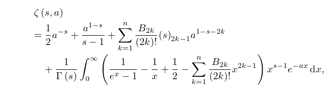
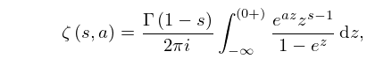
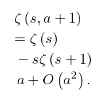
15: 25.11 Hurwitz Zeta Function

… ►

25.11.28 $$\zeta (s,a)=\frac{1}{2}{a}^{-s}+\frac{a^{1-s}}{s-1}+\sum _{k=1}^n\frac{B_{2k}}{(2k)!}{\left(s\right)}_{2k-1}{a}^{1-s-2k}+\frac{1}{\mathrm{\Gamma }\left(s\right)}{\int }_0^{\mathrm{\infty }}\left(\frac{1}{{\mathrm{e}}^x-1}-\frac{1}{x}+\frac{1}{2}-\sum _{k=1}^n\frac{B_{2k}}{(2k)!}{x}^{2k-1}\right)x^{s-1}{\mathrm{e}}^{-ax}dx,$$ $\mathrm{\Re }s>-(2n+1)$, $s\ne 1$, $\mathrm{\Re }a>0$.

ⓘ

Symbols:

$B_n$: Bernoulli numbers, $O\left(x\right)$: order not exceeding, $\mathrm{\Gamma }\left(z\right)$: gamma function, $\zeta (s,a)$: Hurwitz zeta function, ${\left(a\right)}_n$: Pochhammer’s symbol (or shifted factorial), $dx$: differential of $x$ , $\mathrm{e}$: base of natural logarithm, $!$: factorial (as in $n!$), $\int$: integral, $\mathrm{\Re }$: real part, $k$: nonnegative integer, $n$: nonnegative integer, $x$: real variable, $a$: real or complex parameter and $s$: complex variable

Keywords:

improper integral, integral representation

Proof sketch:

Derivable from (25.11.27) by adding and subtracting ${\sum }_{k=1}^n{B}_{2k}{x}^{2k-1}/(2k)!$ in the integrand, using (5.2.1), (5.2.5), and recognizing that ${({\mathrm{e}}^x-1)}^{-1}-x^{-1}+1/2-{\sum }_{k=1}^n{B}_{2k}{x}^{2k-1}/(2k)!=O\left(x^{2n+1}\right)$ as $x\to 0$, demonstrating the region of convergence.

Referenced by:

Erratum (V1.0.9) for Chapters 7, 25

Permalink:

http://dlmf.nist.gov/25.11.E28

Encodings:

pMML, png, TeX

Notational Change (effective with 1.0.9):

We have rewritten the original summation ${\sum }_{k=1}^n\frac{\mathrm{\Gamma }\left(s+2k-1\right)}{\mathrm{\Gamma }\left(s\right)}\frac{B_{2k}}{(2k)!}{a}^{-2k-s+1}$ more concisely as ${\sum }_{k=1}^n\frac{B_{2k}}{(2k)!}{\left(s\right)}_{2k-1}{a}^{1-s-2k}$ using the Pochhammer symbol.

See also:

Annotations for §25.11(vii), §25.11 and Ch.25

… ►

25.11.30 $$\zeta (s,a)=\frac{\mathrm{\Gamma }\left(1-s\right)}{2\pi \mathrm{i}}{\int }_{-\mathrm{\infty }}^{(0+)}\frac{{\mathrm{e}}^{az}{z}^{s-1}}{1-{\mathrm{e}}^z}dz,$$ $s\ne 1$, $\mathrm{\Re }a>0$,

ⓘ

Symbols:

$\mathrm{\Gamma }\left(z\right)$: gamma function, $\zeta (s,a)$: Hurwitz zeta function, $\pi$: the ratio of the circumference of a circle to its diameter, $dx$: differential of $x$ , $\mathrm{e}$: base of natural logarithm, $\mathrm{i}$: imaginary unit, $\int$: integral, $\mathrm{\Re }$: real part, $a$: real or complex parameter, $s$: complex variable and $z$: complex variable

Keywords:

contour integral, integral representation

Source:

Erdélyi et al. (1953a, (1.10.5), p. 25); with $z=-t$

Proof sketch:

This contour integral uses Hankel’s contour Figure 5.9.1. Assume $\mathrm{\Re }s>1$, collapse the integration path onto the negative real axis, apply (25.11.25), followed by analytic continuation for all $s\ne 1$, $\mathrm{\Re }a>0$, since the integrand is analytic in $z$, the convergence at the ends of the path is exponential for all $s\ne -1$ and the Hankel contour can be kept well clear of the singularity at the origin in the $z$-plane.

Referenced by:

§25.11(i)

Permalink:

http://dlmf.nist.gov/25.11.E30

Encodings:

pMML, png, TeX

See also:

Annotations for §25.11(vii), §25.11 and Ch.25

… ►

25.11.41 $$\zeta (s,a+1)=\zeta \left(s\right)-s\zeta \left(s+1\right)a+O\left(a^2\right).$$

ⓘ

Symbols:

$O\left(x\right)$: order not exceeding, $\zeta (s,a)$: Hurwitz zeta function, $\zeta \left(s\right)$: Riemann zeta function, $a$: real or complex parameter and $s$: complex variable

Keywords:

asymptotic approximation

Source:

Apostol (1952, (15), p. 6)

Permalink:

http://dlmf.nist.gov/25.11.E41

Encodings:

pMML, png, TeX

See also:

Annotations for §25.11(xii), §25.11 and Ch.25

…

16: 13.29 Methods of Computation

… ►As described in §3.7(ii), to insure stability the integration path must be chosen in such a way that as we proceed along it the wanted solution grows in magnitude at least as fast as all other solutions of the differential equation. … ►

13.29.4 $$y(n)=1+O\left(n^{-1}\right),$$ $n\to \mathrm{\infty }$.

ⓘ

Symbols:

$O\left(x\right)$: order not exceeding, $n$: nonnegative integer and $y(n)$: solution

Permalink:

http://dlmf.nist.gov/13.29.E4

Encodings:

pMML, png, TeX

See also:

Annotations for §13.29(iv), §13.29(iv), §13.29 and Ch.13

…

17: 3.5 Quadrature

… ►For these cases the integration path may need to be deformed; see §3.5(ix). … ►

§3.5(ix) Other Contour Integrals

… ►For example, steepest descent paths can be used; see §2.4(iv). … ►with saddle point at $t=1$, and when $c=1$ the vertical path intersects the real axis at the saddle point. … ►A special case is the rule for Hilbert transforms (§1.14(v)): …