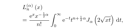
limiting form as a Bessel function

SearchAdvancedHelp

(0.017 seconds)

21—30 of 31 matching pages

21: 9.17 Methods of Computation

… ►Since these expansions diverge, the accuracy they yield is limited by the magnitude of $|z|$. … ►The former reference includes a parallelized version of the method. … ►For details, including the application of a generalized form of Gaussian quadrature, see Gordon (1969, Appendix A) and Schulten et al. (1979). … ►

§9.17(iv) Via Bessel Functions

►In consequence of §9.6(i), algorithms for generating Bessel functions, Hankel functions, and modified Bessel functions (§10.74) can also be applied to $\mathrm{Ai}\left(z\right)$, $\mathrm{Bi}\left(z\right)$, and their derivatives. …

22: 2.8 Differential Equations with a Parameter

… ►Many special functions satisfy an equation of the form …For example, $u$ can be the order of a Bessel function or degree of an orthogonal polynomial. … ►

§2.8(iv) Case III: Simple Pole

… ►For other examples of uniform asymptotic approximations and expansions of special functions in terms of Bessel functions or modified Bessel functions of fixed order see §§13.8(iii), 13.21(i), 13.21(iv), 14.15(i), 14.15(iii), 14.20(vii), 15.12(iii), 18.15(i), 18.15(iv), 18.24, 33.20(iv). … ►For a coalescing turning point and double pole see Boyd and Dunster (1986) and Dunster (1990b); in this case the uniform approximants are Bessel functions of variable order. …

23: 28.28 Integrals, Integral Representations, and Integral Equations

… ►

§28.28(i) Equations with Elementary Kernels

… ►

§28.28(ii) Integrals of Products with Bessel Functions

… ►where the integral is a Cauchy principal value (§1.4(v)). ►

§28.28(iv) Integrals of Products of Mathieu Functions of Integer Order

… ►

§28.28(v) Compendia

…

24: Bibliography C

… ►

Asymptotics and closed form of a generalized incomplete gamma function. J. Comput. Appl. Math. 67 (2), pp. 371–379.

ⓘ

External Links:

ISSN 0377-0427, Document, MathReview, ZentralBlatt

Referenced by:

§8.16.

Encodings:

BibTeX

… ►

Incomplete Hankel and modified Bessel functions: A class of special functions for electromagnetics. IEEE Trans. Antennas and Propagation 52 (12), pp. 3373–3389.

ⓘ

External Links:

ISSN 0018-926X, Document, MathReview (T. Erber), ZentralBlatt

Referenced by:

§10.46.

Encodings:

BibTeX

… ►

Further formulas for calculating approximate values of the zeros of certain combinations of Bessel functions. IEEE Trans. Microwave Theory Tech. 11 (6), pp. 546–547.

ⓘ

External Links:

ISSN 0018-9480, FullText

Referenced by:

§10.21(x).

Encodings:

BibTeX

►

Remarks on the zeros of cross-product Bessel functions. J. Soc. Indust. Appl. Math. 12 (3), pp. 580–587.

ⓘ

External Links:

Document, MathReview (M. J. O. Strutt), ZentralBlatt

Referenced by:

§10.21(x), §10.21(x).

Encodings:

BibTeX

… ►

The analyticity of cross-product Bessel function zeros. Proc. Cambridge Philos. Soc. 62, pp. 215–226.

ⓘ

External Links:

MathReview (R. G. Langebartel), ZentralBlatt

Referenced by:

§10.21(x).

Encodings:

BibTeX

…

25: 3.10 Continued Fractions

… ►However, other continued fractions with the same limit may converge in a much larger domain of the complex plane than the fraction given by (3.10.4) and (3.10.5). … ►A continued fraction of the form … ►For applications to Bessel functions and Whittaker functions (Chapters 10 and 13), see Gargantini and Henrici (1967). … ►A continued fraction of the form … ►can be written in the form …

26: 35.6 Confluent Hypergeometric Functions of Matrix Argument

§35.6 Confluent Hypergeometric Functions of Matrix Argument

►

§35.6(i) Definitions

… ►

Laguerre Form

… ►

§35.6(ii) Properties

… ►

§35.6(iii) Relations to Bessel Functions of Matrix Argument

…

27: 13.23 Integrals

… ►

§13.23(i) Laplace and Mellin Transforms

… ►

§13.23(ii) Fourier Transforms

… ►For additional Hankel transforms and also other Bessel transforms see Erdélyi et al. (1954b, §8.18) and Oberhettinger (1972, §1.16 and 3.4.42–46, 4.4.45–47, 5.94–97). ►

§13.23(iv) Integral Transforms in terms of Whittaker Functions

…

28: 18.18 Sums

… ►In all three cases of Jacobi, Laguerre and Hermite, if $f(x)$ is $L^2$ on the corresponding interval with respect to the corresponding weight function and if $a_n,b_n,d_n$ are given by (18.18.1), (18.18.5), (18.18.7), respectively, then the respective series expansions (18.18.2), (18.18.4), (18.18.6) are valid with the sums converging in $L^2$ sense. … ►See (18.5.11) for the limit case $\lambda \to 0$ of (18.18.16). … ►See (18.17.45) and (18.17.49) for integrated forms of (18.18.22) and (18.18.23), respectively. … ►

Laguerre

… ►For the modified Bessel function $I_{\nu }\left(z\right)$ see §10.25(ii). …

29: 18.10 Integral Representations

… ►Table 18.10.1 gives contour integral representations of the form …Here $C$ is a simple closed contour encircling $z=c$ once in the positive sense. … ►

Laguerre

►

18.10.9 $$L_n^{(\alpha )}\left(x\right)=\frac{{\mathrm{e}}^x{x}^{-\frac{1}{2}\alpha }}{n!}{\int }_0^{\mathrm{\infty }}{\mathrm{e}}^{-t}{t}^{n+\frac{1}{2}\alpha }{J}_{\alpha }\left(2\sqrt{xt}\right)dt,$$ $\alpha >-1$.

ⓘ

Symbols:

$J_{\nu }\left(z\right)$: Bessel function of the first kind, $L_n^{(\alpha )}\left(x\right)$: Laguerre (or generalized Laguerre) polynomial, $dx$: differential of $x$ , $\mathrm{e}$: base of natural logarithm, $!$: factorial (as in $n!$), $\int$: integral, $t$: real variable, $n$: nonnegative integer and $x$: real variable

A&S Ref:

22.10.14

Referenced by:

§18.10(iv)

Permalink:

http://dlmf.nist.gov/18.10.E9

Encodings:

pMML, png, TeX

See also:

Annotations for §18.10(iv), §18.10(iv), §18.10 and Ch.18

►For the Bessel function $J_{\nu }\left(z\right)$ see §10.2(ii). …

30: Errata

… ►The spectral theory of these operators, based on Sturm-Liouville and Liouville normal forms, distribution theory, is now discussed more completely, including linear algebra, matrices, matrices as linear operators, orthonormal expansions, Stieltjes integrals/measures, generating functions. … ►

18.34.1 $$y_n(x;a)={}_2{}^{}F_0^{}(\genfrac{}{}{0pt}{}{-n,n+a-1}{-};-\frac{x}{2})={\left(n+a-1\right)}_n{\left(\frac{x}{2}\right)}^n{}_1{}^{}F_1^{}(\genfrac{}{}{0pt}{}{-n}{-2n-a+2};\frac{2}{x})=n!{\left(-\frac{1}{2}x\right)}^n{L}_n^{(1-a-2n)}\left(2x^{-1}\right)={\left(\frac{1}{2}x\right)}^{1-\frac{1}{2}a}{\mathrm{e}}^{1/x}{W}_{1-\frac{1}{2}a,\frac{1}{2}(a-1)+n}\left(2x^{-1}\right)$$

This equation was updated to include the definition of Bessel polynomials in terms of Laguerre polynomials and the Whittaker confluent hypergeometric function.

… ►

The following additions were made in Chapter 1:

• New subsections, 1.2(v) Matrices, Vectors, Scalar Products, and Norms and 1.2(vi) Square Matrices, with Equations (1.2.27)–(1.2.77).

• The title of this section was changed from “Determinants” to “Determinants, Linear Operators, and Spectral Expansions”. An extra paragraph just below (1.3.7). New subsection, 1.3(iv) Matrices as Linear Operators, with Equations (1.3.20), (1.3.21).

• In 1.4(v), three new paragraphs on Stieltjes integrals/measure, with Equations (1.4.23_1)–(1.4.23_3).

• In Subsection 1.8(i), the title of the paragraph “Bessel’s Inequality” was changed to “Parseval’s Formula”. We give the relation between the real and the complex coefficients, and include more general versions of Parseval’s Formula, Equations (1.8.6_1), (1.8.6_2). The title of Subsection 1.8(iv) was changed from “Transformations” to “Poisson’s Summation Formula”, and we added an extra remark just below (1.8.14).

• New subsection, 1.10(xi) Generating Functions, with Equations (1.10.26)–(1.10.29).

• New subsection, 1.13(viii) Eigenvalues and Eigenfunctions: Sturm-Liouville and Liouville forms, with Equations (1.13.26)–(1.13.31).

• Another form of Parseval’s formula, (1.14.7_5).

• We include several extra remarks and Equations (1.16.3_5), (1.16.9_5). New subsection, 1.16(ix) References for Section 1.16.

• Two extra paragraphs in Subsection 1.17(ii) Integral Representations, with Equations (1.17.12_1), (1.17.12_2); Subsection 1.17(iv) Mathematical Definitions is almost completely rewritten.

• An entire new section, 1.18 Linear Second Order Differential Operators and Eigenfunction Expansions, including new subsections, 1.18(i)–1.18(x), and several equations, (1.18.1)–(1.18.71).

… ►

Just below (33.14.9), the constraint described in the text “ when ,” was removed. In Equation (33.14.13), the constraint ${ϵ}_1,{ϵ}_2>0$ was added. In the line immediately below (33.14.13), it was clarified that $s(ϵ,\mathrm{\ell };r)$ is $\exp \left(-r/n\right)$ times a polynomial in $r/n$, instead of simply a polynomial in $r$. In Equation (33.14.14), a second equality was added which relates ${\varphi }_{n,\mathrm{\ell }}(r)$ to Laguerre polynomials. A sentence was added immediately below (33.14.15) indicating that the functions ${\varphi }_{n,\mathrm{\ell }}$, $n=\mathrm{\ell },\mathrm{\ell }+1,\mathrm{\dots }$, do not form a complete orthonormal system.

… ►

A sentence was added in §8.18(ii) to refer to Nemes and Olde Daalhuis (2016). Originally §8.11(iii) was applicable for real variables $a$ and $x=\lambda a$. It has been extended to allow for complex variables $a$ and $z=\lambda a$ (and we have replaced $x$ with $z$ in the subsection heading and in Equations (8.11.6) and (8.11.7)). Also, we have added two paragraphs after (8.11.9) to replace the original paragraph that appeared there. Furthermore, the interval of validity of (8.11.6) was increased from to the sector , and the interval of validity of (8.11.7) was increased from $\lambda >1$ to the sector $\lambda >1$, $|\mathrm{ph}a|\le \frac{3\pi }{2}-\delta$. A paragraph with reference to Nemes (2016) has been added in §8.11(v), and the sector of validity for (8.11.12) was increased from $|\mathrm{ph}z|\le \pi -\delta$ to $|\mathrm{ph}z|\le 2\pi -\delta$. Two new Subsections 13.6(vii), 13.18(vi), both entitled Coulomb Functions, were added to note the relationship of the Kummer and Whittaker functions to various forms of the Coulomb functions. A sentence was added in both §13.10(vi) and §13.23(v) noting that certain generalized orthogonality can be expressed in terms of Kummer functions.

…