large order
(0.002 seconds)
41—50 of 89 matching pages
41: 13.22 Zeros
…
►Asymptotic approximations to the zeros when the parameters and/or are large can be found by reversion of the uniform approximations provided in §§13.20 and 13.21.
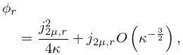
For example, if is fixed and is large, then the th positive zero of is given by
►
13.22.1
…
42: 2.4 Contour Integrals
…
►Except that is now permitted to be complex, with , we assume the same conditions on and also that the Laplace transform in (2.3.8) converges for all sufficiently large values of .
Then
…
►For large
, the asymptotic expansion of may be obtained from (2.4.3) by Haar’s method. This depends on the availability of a comparison function for that has an inverse transform
…If this integral converges uniformly at each limit for all sufficiently large
, then by the Riemann–Lebesgue lemma (§1.8(i))
…
►in which is a large real or complex parameter, and are analytic functions of and continuous in and a second parameter .
…
43: 13.8 Asymptotic Approximations for Large Parameters
§13.8 Asymptotic Approximations for Large Parameters
… ►§13.8(ii) Large and , Fixed and
… ►§13.8(iii) Large
… ► … ►§13.8(iv) Large and
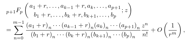
…44: 16.11 Asymptotic Expansions
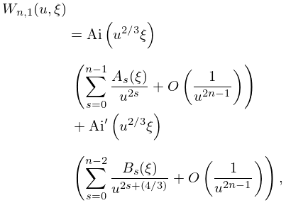
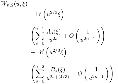
45: 2.8 Differential Equations with a Parameter
46: 10.68 Modulus and Phase Functions
…
►
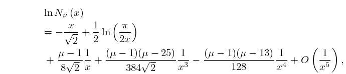
§10.68(iii) Asymptotic Expansions for Large Argument
… ►
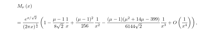
10.68.16
►
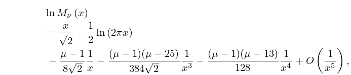
10.68.17
►
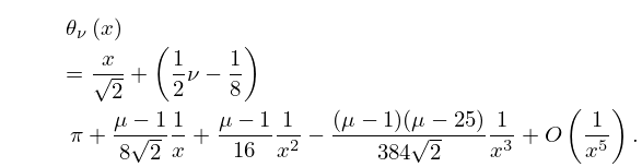
10.68.18
…
►
10.68.20
…
47: 30.11 Radial Spheroidal Wave Functions
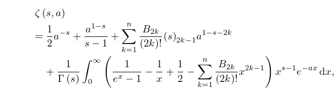
48: 25.11 Hurwitz Zeta Function
…
►
25.11.28
, , .
…
►
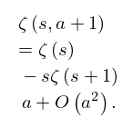
§25.11(xii) -Asymptotic Behavior
… ►
25.11.41
…
►Similarly, as in the sector ,
…
49: 33.10 Limiting Forms for Large or Large
§33.10 Limiting Forms for Large or Large
►§33.10(i) Large
… ►§33.10(ii) Large Positive
… ►§33.10(iii) Large Negative
…50: 27.11 Asymptotic Formulas: Partial Sums
…
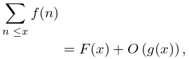
►The behavior of a number-theoretic function for large
is often difficult to determine because the function values can fluctuate considerably as increases.
…
►
27.11.1
►where is a known function of , and represents the error, a function of smaller order than for all in some prescribed range.
…
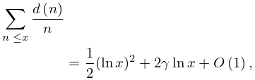
►
27.11.2
…
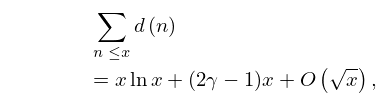
►
27.11.3
…
