inversion formula

(0.003 seconds)

31—40 of 56 matching pages

31: 15.4 Special Cases

… ►

15.4.3

F\left(\tfrac{1}{2},1;\tfrac{3}{2};-z^{2}\right)=z^{-1}\operatorname{arctan}z,

ⓘ

Symbols:: $F\left(\NVar{a},\NVar{b};\NVar{c};\NVar{z}\right)$ or $F\left({\NVar{a},\NVar{b}\atop\NVar{c}};\NVar{z}\right)$ : $={{}_{2}F_{1}}\left(\NVar{a},\NVar{b};\NVar{c};\NVar{z}\right)$ Gauss’ hypergeometric function, $\operatorname{arctan}\NVar{z}$ : arctangent function and $z$ : complex variable
Permalink:: http://dlmf.nist.gov/15.4.E3
Encodings:: pMML, png, TeX
See also:: Annotations for §15.4(i), §15.4 and Ch.15

►

15.4.4

F\left(\tfrac{1}{2},\tfrac{1}{2};\tfrac{3}{2};z^{2}\right)=z^{-1}\operatorname% {arcsin}z,

ⓘ

Symbols:: $F\left(\NVar{a},\NVar{b};\NVar{c};\NVar{z}\right)$ or $F\left({\NVar{a},\NVar{b}\atop\NVar{c}};\NVar{z}\right)$ : $={{}_{2}F_{1}}\left(\NVar{a},\NVar{b};\NVar{c};\NVar{z}\right)$ Gauss’ hypergeometric function, $\operatorname{arcsin}\NVar{z}$ : arcsine function and $z$ : complex variable
Permalink:: http://dlmf.nist.gov/15.4.E4
Encodings:: pMML, png, TeX
See also:: Annotations for §15.4(i), §15.4 and Ch.15

…

33: 6.10 Other Series Expansions

… ►

§6.10(i) Inverse Factorial Series

… ►For a more general result (incomplete gamma function), and also for a result for the logarithmic integral, see Nielsen (1906a, p. 283: Formula (3) is incorrect). …

34: 19.11 Addition Theorems

… ►

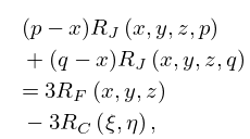
§19.11(i) General Formulas

… ►

19.11.5

\Pi\left(\theta,\alpha^{2},k\right)+\Pi\left(\phi,\alpha^{2},k\right)=\Pi\left% (\psi,\alpha^{2},k\right)-\alpha^{2}R_{C}\left(\gamma-\delta,\gamma\right),

ⓘ

Symbols:: $R_{C}\left(\NVar{x},\NVar{y}\right)$ : Carlson’s combination of inverse circular and inverse hyperbolic functions, $\Pi\left(\NVar{\phi},\NVar{\alpha}^{2},\NVar{k}\right)$ : Legendre’s incomplete elliptic integral of the third kind, $\phi$ : real or complex argument, $k$ : real or complex modulus, $\alpha^{2}$ : real or complex parameter, $\theta$ : amplitude, $\psi$ : angle, $\gamma$ and $\delta$
Referenced by:: §19.11(i), §19.11(i), Erratum (V1.0.24) for Subsection 19.11(i)
Permalink:: http://dlmf.nist.gov/19.11.E5
Encodings:: pMML, png, TeX
See also:: Annotations for §19.11(i), §19.11 and Ch.19

… ►

19.11.6_5

R_{C}\left(\gamma-\delta,\gamma\right)=\frac{-1}{\sqrt{\delta}}\operatorname{% arctan}\left(\frac{\sqrt{\delta}\sin\theta\sin\phi\sin\psi}{\alpha^{2}-1-% \alpha^{2}\cos\theta\cos\phi\cos\psi}\right).

ⓘ

Symbols:: $R_{C}\left(\NVar{x},\NVar{y}\right)$ : Carlson’s combination of inverse circular and inverse hyperbolic functions, $\cos\NVar{z}$ : cosine function, $\operatorname{arctan}\NVar{z}$ : arctangent function, $\sin\NVar{z}$ : sine function, $\phi$ : real or complex argument, $\alpha^{2}$ : real or complex parameter, $\theta$ : amplitude, $\psi$ : angle, $\gamma$ and $\delta$
Referenced by:: §19.11(i), Erratum (V1.0.28) for Equations (15.2.3_5), (19.11.6_5)
Permalink:: http://dlmf.nist.gov/19.11.E6_5
Encodings:: pMML, png, TeX
Clarification (effective with 1.0.28):: This equation was given a number.
See also:: Annotations for §19.11(i), §19.11 and Ch.19

… ►

§19.11(iii) Duplication Formulas

… ►

19.11.16

\Pi\left(\psi,\alpha^{2},k\right)=2\Pi\left(\theta,\alpha^{2},k\right)+\alpha^% {2}R_{C}\left(\gamma-\delta,\gamma\right),

ⓘ

Symbols:: $R_{C}\left(\NVar{x},\NVar{y}\right)$ : Carlson’s combination of inverse circular and inverse hyperbolic functions, $\Pi\left(\NVar{\phi},\NVar{\alpha}^{2},\NVar{k}\right)$ : Legendre’s incomplete elliptic integral of the third kind, $k$ : real or complex modulus, $\alpha^{2}$ : real or complex parameter, $\theta$ : amplitude, $\delta$ , $\psi$ : angle and $\gamma$
Permalink:: http://dlmf.nist.gov/19.11.E16
Encodings:: pMML, png, TeX
See also:: Annotations for §19.11(iii), §19.11 and Ch.19

…

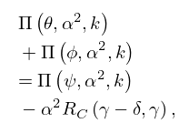
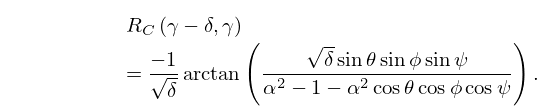
35: 19.21 Connection Formulas

§19.21 Connection Formulas

… ►The complete cases of

R_{F}

and

R_{G}

have connection formulas resulting from those for the Gauss hypergeometric function (Erdélyi et al. (1953a, §2.9)). … ►Connection formulas for

R_{-a}\left(\mathbf{b};\mathbf{z}\right)

are given in Carlson (1977b, pp. 99, 101, and 123–124). … ►

19.21.12

(p-x)R_{J}\left(x,y,z,p\right)+(q-x)R_{J}\left(x,y,z,q\right)=3R_{F}\left(x,y,% z\right)-3R_{C}\left(\xi,\eta\right),

ⓘ

Symbols:: $R_{C}\left(\NVar{x},\NVar{y}\right)$ : Carlson’s combination of inverse circular and inverse hyperbolic functions, $R_{F}\left(\NVar{x},\NVar{y},\NVar{z}\right)$ : symmetric elliptic integral of first kind, $R_{J}\left(\NVar{x},\NVar{y},\NVar{z},\NVar{p}\right)$ : symmetric elliptic integral of third kind, $\xi$ and $\eta$
Referenced by:: §19.15, §19.20(iii), §19.21(iii), §19.25(i), §19.26(i)
Permalink:: http://dlmf.nist.gov/19.21.E12
Encodings:: pMML, png, TeX
See also:: Annotations for §19.21(iii), §19.21 and Ch.19

…

36: 18.3 Definitions

… ►

As given by a Rodrigues formula (18.5.5).

… ►For representations of the polynomials in Table 18.3.1 by Rodrigues formulas, see §18.5(ii). … ►In this chapter, formulas for the Chebyshev polynomials of the second, third, and fourth kinds will not be given as extensively as those of the first kind. However, most of these formulas can be obtained by specialization of formulas for Jacobi polynomials, via (18.7.4)–(18.7.6). … ►Formula (18.3.1) can be understood as a Gauss-Chebyshev quadrature, see (3.5.22), (3.5.23). …

37: 10.22 Integrals

… ►

10.22.59

\int_{0}^{\infty}e^{ibt}J_{\mu}\left(at\right)\,\mathrm{d}t=\begin{cases}% \dfrac{\exp\left(i\mu\operatorname{arcsin}\left(b/a\right)\right)}{(a^{2}-b^{2% })^{\frac{1}{2}}},&0\leq b<a,\\ \dfrac{ia^{\mu}\exp\left(\frac{1}{2}\mu\pi i\right)}{(b^{2}-a^{2})^{\frac{1}{2% }}\left(b+(b^{2}-a^{2})^{\frac{1}{2}}\right)^{\mu}},&0<a<b.\end{cases}

ⓘ

Symbols:: $J_{\NVar{\nu}}\left(\NVar{z}\right)$ : Bessel function of the first kind, $\pi$ : the ratio of the circumference of a circle to its diameter, $\,\mathrm{d}\NVar{x}$ : differential of $x$ , $\exp\NVar{z}$ : exponential function, $\mathrm{e}$ : base of natural logarithm, $\mathrm{i}$ : imaginary unit, $\int$ : integral and $\operatorname{arcsin}\NVar{z}$ : arcsine function
A&S Ref:: 11.4.37, 11.4.38
Referenced by:: §10.22(iv)
Permalink:: http://dlmf.nist.gov/10.22.E59
Encodings:: pMML, png, TeX
See also:: Annotations for §10.22(iv), §10.22(iv), §10.22 and Ch.10

►

10.22.60

\int_{0}^{\infty}e^{ibt}Y_{0}\left(at\right)\,\mathrm{d}t=\begin{cases}(2i/\pi% )(a^{2}-b^{2})^{-\frac{1}{2}}\operatorname{arcsin}\left(b/a\right),&0\leq b<a,% \\ (b^{2}-a^{2})^{-\frac{1}{2}}\left(-1+\dfrac{2i}{\pi}\ln\left(\dfrac{a}{b+(b^{2% }-a^{2})^{\frac{1}{2}}}\right)\right),&0<a<b.\end{cases}

ⓘ

Symbols:: $Y_{\NVar{\nu}}\left(\NVar{z}\right)$ : Bessel function of the second kind, $\pi$ : the ratio of the circumference of a circle to its diameter, $\,\mathrm{d}\NVar{x}$ : differential of $x$ , $\mathrm{e}$ : base of natural logarithm, $\mathrm{i}$ : imaginary unit, $\int$ : integral, $\operatorname{arcsin}\NVar{z}$ : arcsine function and $\ln\NVar{z}$ : principal branch of logarithm function
A&S Ref:: 11.4.40
Referenced by:: §10.22(iv)
Permalink:: http://dlmf.nist.gov/10.22.E60
Encodings:: pMML, png, TeX
See also:: Annotations for §10.22(iv), §10.22(iv), §10.22 and Ch.10

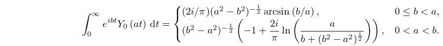
… ►Hankel’s inversion theorem is given by ►

10.22.77

f(y)=\int_{0}^{\infty}g(x)J_{\nu}\left(xy\right)(xy)^{\frac{1}{2}}\,\mathrm{d}x.

ⓘ

Symbols:: $J_{\NVar{\nu}}\left(\NVar{z}\right)$ : Bessel function of the first kind, $\,\mathrm{d}\NVar{x}$ : differential of $x$ , $\int$ : integral, $x$ : real variable, $y$ : real variable, $\nu$ : complex parameter, $f(x)$ : function and $g(y)$ : function
Referenced by:: §1.18(vi), §10.22(v)
Permalink:: http://dlmf.nist.gov/10.22.E77
Encodings:: pMML, png, TeX
See also:: Annotations for §10.22(v), §10.22 and Ch.10

… ►The following two formulas are generalizations of the Hankel transform. …

38: 1.14 Integral Transforms

… ►

Inversion

… ►

Inversion

… ►

Inversion

… ►

Inversion

… ►

Inversion

…

39: 28.2 Definitions and Basic Properties

… ►The solutions of (28.2.16) are given by

\nu=\pi^{-1}\operatorname{arccos}\left(w_{\mbox{\tiny I}}(\pi;a,q)\right)

. If the inverse cosine takes its principal value (§4.23(ii)), then

\nu=\widehat{\nu}

, where

0\leq\Re\widehat{\nu}\leq 1

. … ►(28.2.9), (28.2.16), and (28.2.7) give for each solution

w(z)

of (28.2.1) the connection formula …

40: Bibliography J

… ►

E. Jahnke and F. Emde (1945) Tables of Functions with Formulae and Curves. 4th edition, Dover Publications, New York.

ⓘ

Notes:: Contains corrections and enlargements of earlier editions. Originally published by B. G. Teubner, Leipzig, in 1933. In German and English.
External Links:: MathReview, ZentralBlatt
Referenced by:: 2nd item, §20.15, §5.1, Notations P, E. Jahnke, F. Emde, and F. Lösch (1966).
Encodings:: BibTeX

… ►

D. J. Jeffrey, R. M. Corless, D. E. G. Hare, and D. E. Knuth (1995) Sur l’inversion de

y^{\alpha}e^{y}

au moyen des nombres de Stirling associés. C. R. Acad. Sci. Paris Sér. I Math. 320 (12), pp. 1449–1452.

ⓘ

External Links:: ISSN 0764-4442, MathReview (F. Beukers), ZentralBlatt
Referenced by:: (4.13.10).
Encodings:: BibTeX

… ►

X.-S. Jin and R. Wong (1999) Asymptotic formulas for the zeros of the Meixner polynomials. J. Approx. Theory 96 (2), pp. 281–300.

ⓘ

External Links:: ISSN 0021-9045, Document, MathReview (N. Hayek Calil), ZentralBlatt
Referenced by:: §18.24.
Encodings:: BibTeX

… ►

F. Johansson (2012) Efficient implementation of the Hardy-Ramanujan-Rademacher formula. LMS J. Comput. Math. 15, pp. 341–359.

ⓘ

External Links:: ISSN 1461-1570, Document, Link, MathReview (Tim Huber), ZentralBlatt
Referenced by:: §27.20.
Encodings:: BibTeX

…

inversion formula

31—40 of 56 matching pages

31: 15.4 Special Cases

32: 3.3 Interpolation

Three-Point Formula

Four-Point Formula

Five-Point Formula

Six-Point Formula

§3.3(v) Inverse Interpolation

33: 6.10 Other Series Expansions

§6.10(i) Inverse Factorial Series

34: 19.11 Addition Theorems

§19.11(i) General Formulas

§19.11(iii) Duplication Formulas

35: 19.21 Connection Formulas

§19.21 Connection Formulas

36: 18.3 Definitions

37: 10.22 Integrals

38: 1.14 Integral Transforms

Inversion

Inversion

Inversion

Inversion

Inversion

39: 28.2 Definitions and Basic Properties

40: Bibliography J