interval arithmetic

♦ 11—20 of 24 matching pages ♦

(0.002 seconds)

11—20 of 24 matching pages

11: Bibliography M

… ►

mpmath (free python library)

ⓘ

Notes:: Mpmath is a pure-Python library for multiprecision floating-point arithmetic. It provides an extensive set of transcendental functions, unlimited exponent sizes, complex numbers, interval arithmetic, numerical integration and differentiation, root-finding, linear algebra, and much more.
External Links:: mpmath
Referenced by:: § ‣ Software Cross Index, § ‣ Software Cross Index, § ‣ Software Cross Index, § ‣ Software Cross Index, § ‣ Software Cross Index, § ‣ Software Cross Index, § ‣ Software Cross Index, § ‣ Software Cross Index, § ‣ Software Cross Index, § ‣ Software Cross Index, § ‣ Software Cross Index, § ‣ Software Cross Index, § ‣ Software Cross Index, § ‣ Software Cross Index, § ‣ Software Cross Index, § ‣ Software Cross Index, § ‣ Software Cross Index, § ‣ Software Cross Index, § ‣ Software Cross Index, § ‣ Software Cross Index, § ‣ Software Cross Index, § ‣ Software Cross Index, § ‣ Software Cross Index, § ‣ Software Cross Index, § ‣ Software Cross Index, § ‣ Software Cross Index, § ‣ Software Cross Index, § ‣ Software Cross Index, § ‣ Software Cross Index, § ‣ Software Cross Index, § ‣ Software Cross Index, § ‣ Software Cross Index, § ‣ Software Cross Index, § ‣ Software Cross Index, § ‣ Software Cross Index, § ‣ Software Cross Index, § ‣ Software Cross Index, § ‣ Software Cross Index, § ‣ Software Cross Index, § ‣ Software Cross Index, § ‣ Software Cross Index, § ‣ Software Cross Index, § ‣ Software Cross Index, § ‣ Software Cross Index, § ‣ Software Cross Index, § ‣ Software Cross Index, § ‣ Software Cross Index, § ‣ Software Cross Index, § ‣ Software Cross Index, § ‣ Software Cross Index, § ‣ Software Cross Index, § ‣ Software Cross Index, § ‣ Software Cross Index, § ‣ Software Cross Index, § ‣ Software Cross Index, § ‣ Software Cross Index, § ‣ Software Cross Index, § ‣ Software Cross Index, § ‣ Software Cross Index, § ‣ Software Cross Index, § ‣ Software Cross Index, § ‣ Software Cross Index, § ‣ Software Cross Index, § ‣ Software Cross Index.
Encodings:: BibTeX

…

In ¶IEEE Standard (in §3.1(i)), the description was modified to reflect the most recent IEEE 754-2019 Floating-Point Arithmetic Standard IEEE (2019). In the new standard, single, double and quad floating-point precisions are replaced with new standard names of binary32, binary64 and binary128. Figure 3.1.1 has been expanded to include the binary128 floating-point memory positions and the caption has been updated using the terminology of the 2019 standard. A sentence at the end of Subsection 3.1(ii) has been added referring readers to the IEEE Standards for Interval Arithmetic IEEE (2015, 2018).

Suggested by Nicola Torracca.

…

13: 22.20 Methods of Computation

… ►

§22.20(ii) Arithmetic-Geometric Mean

… ►Then as

n\to\infty

sequences

\{a_{n}\}

\{b_{n}\}

converge to a common limit

M=M\left(a_{0},b_{0}\right)

, the arithmetic-geometric mean of

a_{0},b_{0}

. … ►The rate of convergence is similar to that for the arithmetic-geometric mean. … ►using the arithmetic-geometric mean. … ►Alternatively, Sala (1989) shows how to apply the arithmetic-geometric mean to compute

\operatorname{am}\left(x,k\right)

. …

14: 15.17 Mathematical Applications

… ►First, as spherical functions on noncompact Riemannian symmetric spaces of rank one, but also as associated spherical functions, intertwining functions, matrix elements of SL

(2,\mathbb{R})

, and spherical functions on certain nonsymmetric Gelfand pairs. … ►Quadratic transformations give insight into the relation of elliptic integrals to the arithmetic-geometric mean (§19.22(ii)). … …

15: 19.8 Quadratic Transformations

… ►

§19.8(i) Gauss’s Arithmetic-Geometric Mean (AGM)

… ►As

n\to\infty

a_{n}

and

g_{n}

converge to a common limit

M\left(a_{0},g_{0}\right)

called the AGM (Arithmetic-Geometric Mean) of

a_{0}

and

g_{0}

. …showing that the convergence of

c_{n}

to 0 and of

a_{n}

and

g_{n}

M\left(a_{0},g_{0}\right)

is quadratic in each case. … ►

19.8.5

K\left(k\right)=\frac{\pi}{2M\left(1,k^{\prime}\right)},

-\infty<k^{2}<1

ⓘ

Symbols:: $M\left(\NVar{a},\NVar{g}\right)$ : arithmetic-geometric mean, $\pi$ : the ratio of the circumference of a circle to its diameter, $K\left(\NVar{k}\right)$ : Legendre’s complete elliptic integral of the first kind, $k$ : real or complex modulus and $k^{\prime}$ : complementary modulus
Permalink:: http://dlmf.nist.gov/19.8.E5
Encodings:: pMML, png, TeX
See also:: Annotations for §19.8(i), §19.8 and Ch.19

… ►Again,

p_{n}

and

\varepsilon_{n}

converge quadratically to

M\left(a_{0},g_{0}\right)

and 0, respectively, and

Q_{n}

converges to 0 faster than quadratically. …

16: Bibliography C

… ►

M. Carmignani and A. Tortorici Macaluso (1985) Calcolo delle funzioni speciali

\Gamma(x)

\log\Gamma(x)

\beta(x,y)

\operatorname{erf}(x)

\operatorname{erfc}(x)

alle alte precisioni. Atti Accad. Sci. Lett. Arti Palermo Ser. (5) 2(1981/82) (1), pp. 7–25 (Italian).

ⓘ

Notes:: Translated title: Computation of the special functions $\Gamma(x),\;{\rm log}\,\Gamma(x),\;\beta(x,y),\;{\rm erf}\,(x),\;{\rm erfc}\,(x)$ to a high degree of precision
External Links:: MathReview, ZentralBlatt
Referenced by:: §5.24(ii).
Encodings:: BibTeX

… ►

C. W. Clenshaw, F. W. J. Olver, and P. R. Turner (1989) Level-Index Arithmetic: An Introductory Survey. In Numerical Analysis and Parallel Processing (Lancaster, 1987), P. R. Turner (Ed.), Lecture Notes in Math., Vol. 1397, pp. 95–168.

ⓘ

External Links:: MathReview Entry, ZentralBlatt
Referenced by:: §3.1(iv).
Encodings:: BibTeX

… ►

CoStLy (free C-XSC library)

ⓘ

Notes:: Complex interval standard function library. For details see Neher (2007)
External Links:: CoStLy
Referenced by:: § ‣ Software Cross Index, M. Neher (2007).
Encodings:: BibTeX

… ►

D. A. Cox (1984) The arithmetic-geometric mean of Gauss. Enseign. Math. (2) 30 (3-4), pp. 275–330.

ⓘ

External Links:: ISSN 0013-8584, MathReview (Bruce C. Berndt), ZentralBlatt
Referenced by:: §19.8(i).
Encodings:: BibTeX

►

D. A. Cox (1985) Gauss and the arithmetic-geometric mean. Notices Amer. Math. Soc. 32 (2), pp. 147–151.

ⓘ

External Links:: ISSN 0002-9920, MathReview (Willard Parker)
Referenced by:: §19.8(i).
Encodings:: BibTeX

…

17: 18.39 Applications in the Physical Sciences

… ►where the orthogonality measure is now

\,\mathrm{d}r

r\in[0,\infty).

… ►Orthogonality, with measure

\,\mathrm{d}r

for

r\in[0,\infty)

, for fixed

l

… ►normalized with measure

r^{2}\,\mathrm{d}r

r\in[0,\infty)

. … ►A major difficulty in such calculations, loss of precision, is addressed in Gautschi (2009) where use of variable precision arithmetic is discussed and employed. … ►which maps

\epsilon\in[0,\infty)

onto

x\in[-1,1]

. …

18: 23.22 Methods of Computation

… ►

(a)

In the general case, given by $cd\neq 0$ , we compute the roots $\alpha$ , $\beta$ , $\gamma$ , say, of the cubic equation $4t^{3}-ct-d=0$ ; see §1.11(iii). These roots are necessarily distinct and represent $e_{1}$ , $e_{2}$ , $e_{3}$ in some order.

If $c$ and $d$ are real, and the discriminant is positive, that is $c^{3}-27d^{2}>0$ , then $e_{1}$ , $e_{2}$ , $e_{3}$ can be identified via (23.5.1), and $k^{2}$ , ${k^{\prime}}^{2}$ obtained from (23.6.16).

If $c^{3}-27d^{2}<0$ , or $c$ and $d$ are not both real, then we label $\alpha$ , $\beta$ , $\gamma$ so that the triangle with vertices $\alpha$ , $\beta$ , $\gamma$ is positively oriented and $[\alpha,\gamma]$ is its longest side (chosen arbitrarily if there is more than one). In particular, if $\alpha$ , $\beta$ , $\gamma$ are collinear, then we label them so that $\beta$ is on the line segment $(\alpha,\gamma)$ . In consequence, $k^{2}=(\beta-\gamma)/(\alpha-\gamma)$ , ${k^{\prime}}^{2}=(\alpha-\beta)/(\alpha-\gamma)$ satisfy $\Im k^{2}\geq 0\geq\Im{k^{\prime}}^{2}$ (with strict inequality unless $\alpha$ , $\beta$ , $\gamma$ are collinear); also $|k^{2}|$ , $|{k^{\prime}}^{2}|\leq 1$ .

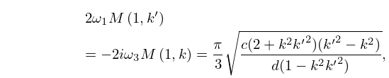
Finally, on taking the principal square roots of $k^{2}$ and ${k^{\prime}}^{2}$ we obtain values for $k$ and $k^{\prime}$ that lie in the 1st and 4th quadrants, respectively, and $2\omega_{1}$ , $2\omega_{3}$ are given by

23.22.1

2\omega_{1}M\left(1,k^{\prime}\right)=-2i\omega_{3}M\left(1,k\right)=\frac{\pi% }{3}\sqrt{\frac{c(2+k^{2}{k^{\prime}}^{2})({k^{\prime}}^{2}-k^{2})}{d(1-k^{2}{% k^{\prime}}^{2})}},

ⓘ

Symbols:: $M\left(\NVar{a},\NVar{g}\right)$ : arithmetic-geometric mean, $\pi$ : the ratio of the circumference of a circle to its diameter, $\mathrm{i}$ : imaginary unit, $\omega_{1}$ , $\omega_{3}$ , $\omega_{2}=-\omega_{1}-\omega_{3}$ : lattice generators, $k$ : modulus and $k^{\prime}$ : complementary modulus
Proof sketch:: Combine (23.6.16), (23.6.17), (22.20.6), (23.3.5)–(23.3.7), and use analytical continuation.
Referenced by:: §23.22(ii)
Permalink:: http://dlmf.nist.gov/23.22.E1
Encodings:: pMML, png, TeX
See also:: Annotations for §23.22(ii), §23.22(ii), §23.22 and Ch.23

where $M$ denotes the arithmetic-geometric mean (see §§19.8(i) and 22.20(ii)). This process yields 2 possible pairs ( $2\omega_{1}$ , $2\omega_{3}$ ), corresponding to the 2 possible choices of the square root.

…

19: 1.7 Inequalities

… ►

§1.7(iii) Means

… ►

1.7.7

H\leq G\leq A,

ⓘ

Symbols:: $A$ : arithmetic mean, $G$ : geometric mean and $H$ : harmonic mean
A&S Ref:: 3.2.1
Permalink:: http://dlmf.nist.gov/1.7.E7
Encodings:: pMML, png, TeX
See also:: Annotations for §1.7(iii), §1.7 and Ch.1

… ►For

f

integrable on

[0,1]

a<f(x)<b

, and

\phi

convex on

(a,b)

(§1.4(viii)), …

20: 1.9 Calculus of a Complex Variable

… ►It is single-valued on

\mathbb{C}\setminus\{0\}

, except on the interval

(-\infty,0)

where it is discontinuous and two-valued. … ►

Arithmetic Operations

… ►A function of two complex variables

f(z,w)

is continuous at

(z_{0},w_{0})

\lim\limits_{(z,w)\to(z_{0},w_{0})}f(z,w)=f(z_{0},w_{0})

; compare (1.5.1) and (1.5.2). … ►at

(x,y)

. … ►Let

(a,b)

be a finite or infinite interval, and

f_{0}(t),f_{1}(t),\dots

be real or complex continuous functions,

t\in(a,b)

. …