integral equations

SearchAdvancedHelp

(0.009 seconds)

41—50 of 215 matching pages

41: 24.7 Integral Representations

§24.7 Integral Representations

►

§24.7(i) Bernoulli and Euler Numbers

… ►

§24.7(ii) Bernoulli and Euler Polynomials

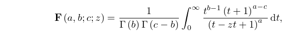
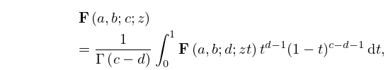
►The following four equations hold for . … ►

Mellin–Barnes Integral

…

42: 9.15 Mathematical Applications

… ►Airy functions play an indispensable role in the construction of uniform asymptotic expansions for contour integrals with coalescing saddle points, and for solutions of linear second-order ordinary differential equations with a simple turning point. …

43: 22.14 Integrals

… ►

22.14.16 $${\int }_0^{K\left(k\right)}\ln \left(\mathrm{sn}(t,k)\right)dt=-\frac{\pi }{4}{K}^{\prime }\left(k\right)-\frac{1}{2}K\left(k\right)\ln k,$$

ⓘ

Symbols:

$\mathrm{sn}(z,k)$: Jacobian elliptic function, $\pi$: the ratio of the circumference of a circle to its diameter, $K^{\prime }\left(k\right)$: Legendre’s complementary complete elliptic integral of the first kind, $K\left(k\right)$: Legendre’s complete elliptic integral of the first kind, $dx$: differential of $x$ , $\int$: integral, $\ln z$: principal branch of logarithm function and $k$: modulus

Referenced by:

Erratum (V1.0.28) for Equations (22.14.16), (22.14.17)

Permalink:

http://dlmf.nist.gov/22.14.E16

Encodings:

pMML, png, TeX

Correction (effective with 1.0.28):

Originally, a factor of $\pi$ was missing from the term containing the $\frac{1}{4}{K}^{\prime }\left(k\right)$.

Suggested 2020-08-06 by Fred Hucht

See also:

Annotations for §22.14(iv), §22.14 and Ch.22

►

22.14.17 $${\int }_0^{K\left(k\right)}\ln \left(\mathrm{cn}(t,k)\right)dt=-\frac{\pi }{4}{K}^{\prime }\left(k\right)+\frac{1}{2}K\left(k\right)\ln \left(k^{\prime }/k\right),$$

ⓘ

Symbols:

$\mathrm{cn}(z,k)$: Jacobian elliptic function, $\pi$: the ratio of the circumference of a circle to its diameter, $K^{\prime }\left(k\right)$: Legendre’s complementary complete elliptic integral of the first kind, $K\left(k\right)$: Legendre’s complete elliptic integral of the first kind, $dx$: differential of $x$ , $\int$: integral, $\ln z$: principal branch of logarithm function, $k$: modulus and $k^{\prime }$: complementary modulus

Referenced by:

Erratum (V1.0.28) for Equations (22.14.16), (22.14.17)

Permalink:

http://dlmf.nist.gov/22.14.E17

Encodings:

pMML, png, TeX

Correction (effective with 1.0.28):

Originally, a factor of $\pi$ was missing from the term containing the $\frac{1}{4}{K}^{\prime }\left(k\right)$.

Suggested 2020-08-06 by Fred Hucht

See also:

Annotations for §22.14(iv), §22.14 and Ch.22

…

44: 10.71 Integrals

§10.71 Integrals

►

§10.71(i) Indefinite Integrals

… ►

§10.71(ii) Definite Integrals

… ►

§10.71(iii) Compendia

… ►

45: 28.30 Expansions in Series of Eigenfunctions

… ►

28.30.2 $$\frac{1}{2\pi }{\int }_0^{2\pi }{w}_m(x)w_n(x)dx={\delta }_{m,n}.$$

ⓘ

Symbols:

${\delta }_{j,k}$: Kronecker delta, $\pi$: the ratio of the circumference of a circle to its diameter, $dx$: differential of $x$ , $\int$: integral, $m$: integer, $n$: integer, $x$: real variable and $w(z)$: Mathieu’s equation solution

Permalink:

http://dlmf.nist.gov/28.30.E2

Encodings:

pMML, png, TeX

See also:

Annotations for §28.30(i), §28.30 and Ch.28

… ►

28.30.4 $$f_m=\frac{1}{2\pi }{\int }_0^{2\pi }f(x)w_m(x)dx.$$

ⓘ

Symbols:

$\pi$: the ratio of the circumference of a circle to its diameter, $dx$: differential of $x$ , $\int$: integral, $m$: integer, $x$: real variable and $w(z)$: Mathieu’s equation solution

Permalink:

http://dlmf.nist.gov/28.30.E4

Encodings:

pMML, png, TeX

See also:

Annotations for §28.30(i), §28.30 and Ch.28

…

46: Bibliography G

… ►

Sur les équations différentielles du second ordre et du premier degré dont l’intégrale générale est a points critiques fixes. Acta Math. 33 (1), pp. 1–55.

ⓘ

External Links:

ISSN 0001-5962, Document, MathReview Entry, ZentralBlatt

Referenced by:

§32.10(ii), §32.10(iv), §32.7(ii).

Encodings:

BibTeX

… ►

The solution of Cauchy’s problem for two totally hyperbolic linear differential equations by means of Riesz integrals. Ann. of Math. (2) 48 (4), pp. 785–826.

ⓘ

External Links:

FullText, MathReview (E. T. Copson), ZentralBlatt

Referenced by:

§35.2, §35.3(ii).

Encodings:

BibTeX

… ►

Sur l’équation différentielle linéaire, qui admet pour intégrale la série hypergéométrique. Ann. Sci. École Norm. Sup. (2) 10, pp. 3–142 (French).

ⓘ

External Links:

ISSN 0012-9593, MathReview Entry, ZentralBlatt

Referenced by:

§15.8(v), §15.8(v).

Encodings:

BibTeX

…

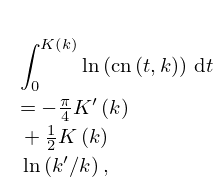
47: 19.16 Definitions

… ►

19.16.9 $$R_{-a}(𝐛;𝐳)=\frac{1}{\mathrm{B}(a,a^{\prime })}{\int }_0^{\mathrm{\infty }}{t}^{a^{\prime }-1}\prod _{j=1}^n{(t+z_j)}^{-b_j}dt=\frac{1}{\mathrm{B}(a,a^{\prime })}{\int }_0^{\mathrm{\infty }}{t}^{a-1}\prod _{j=1}^n{(1+t{z}_j)}^{-b_j}dt,$$ $b_1+\mathrm{\cdots }+b_n>a>0$, $b_j\in ℝ$, $z_j\in ℂ\setminus (-\mathrm{\infty },0]$,

ⓘ

Defines:

$R_{-a}(b_1,\mathrm{\dots },b_n;z_1,\mathrm{\dots },z_n)$ or $R_{-a}(𝐛;𝐳)$: multivariate hypergeometric function

Symbols:

$\mathrm{B}(a,b)$: beta function, $ℂ$: complex plane, $dx$: differential of $x$ , $\in$: element of, $\int$: integral, $(a,b]$: half-closed interval, $ℝ$: real line, $\setminus$: set subtraction and $n$: nonnegative integer

Referenced by:

§19.16(ii), §19.16(ii), §19.19, §19.20(iv), Erratum (V1.0.18) for Equation (19.16.9)

Permalink:

http://dlmf.nist.gov/19.16.E9

Encodings:

pMML, png, TeX

Clarification (effective with 1.0.18):

The constraint $a,a^{\prime }>0$, was replaced with $b_1+\mathrm{\cdots }+b_n>a>0$, $b_j\in ℝ$. It therefore follows from (19.16.10) that $a^{\prime }>0$.

Suggested 2017-07-25 by Bastien Roucariès

See also:

Annotations for §19.16(ii), §19.16 and Ch.19

…

48: 15.6 Integral Representations

… ►

15.6.1 $$𝐅(a,b;c;z)=\frac{1}{\mathrm{\Gamma }\left(b\right)\mathrm{\Gamma }\left(c-b\right)}{\int }_0^1\frac{t^{b-1}{(1-t)}^{c-b-1}}{{(1-zt)}^a}dt,$$ ; $\mathrm{\Re }c>\mathrm{\Re }b>0$.

ⓘ

Symbols:

$\mathrm{\Gamma }\left(z\right)$: gamma function, $\pi$: the ratio of the circumference of a circle to its diameter, $dx$: differential of $x$ , $\int$: integral, $\mathrm{ph}$: phase, $\mathrm{\Re }$: real part, $𝐅(a,b;c;z)$ or $𝐅(\genfrac{}{}{0pt}{}{a,b}{c};z)$: $={}_2{}^{}𝐅_1^{}(a,b;c;z)$ Olver’s hypergeometric function, $z$: complex variable, $a$: real or complex parameter, $b$: real or complex parameter and $c$: real or complex parameter

Keywords:

Mellin transform

Referenced by:

§15.19(iii), (15.4.34), §15.6, §15.6, Erratum (V1.0.23) for Equations (15.6.1)–(15.6.9), Erratum (V1.0.23) for Equations (15.6.1)–(15.6.9)

Permalink:

http://dlmf.nist.gov/15.6.E1

Encodings:

pMML, png, TeX

Addition (effective with 1.0.23):

The Olver hypergeometric function $𝐅(a,b;c;z)$, previously omitted from the left-hand side to make the formula more concise, has been added. The constraint , originally mentioned in the text, has been directly added to the formula.

See also:

Annotations for §15.6 and Ch.15

… ►

15.6.2_5 $$𝐅(a,b;c;z)=\frac{1}{\mathrm{\Gamma }\left(b\right)\mathrm{\Gamma }\left(c-b\right)}{\int }_0^{\mathrm{\infty }}\frac{t^{b-1}{\left(t+1\right)}^{a-c}}{{\left(t-zt+1\right)}^a}dt,$$ ; $\mathrm{\Re }c>\mathrm{\Re }b>0$.

ⓘ

Symbols:

$\mathrm{\Gamma }\left(z\right)$: gamma function, $\pi$: the ratio of the circumference of a circle to its diameter, $dx$: differential of $x$ , $\int$: integral, $\mathrm{ph}$: phase, $\mathrm{\Re }$: real part, $𝐅(a,b;c;z)$ or $𝐅(\genfrac{}{}{0pt}{}{a,b}{c};z)$: $={}_2{}^{}𝐅_1^{}(a,b;c;z)$ Olver’s hypergeometric function, $z$: complex variable, $a$: real or complex parameter, $b$: real or complex parameter and $c$: real or complex parameter

Keywords:

Mellin transform

Referenced by:

§15.6, Erratum (V1.1.5) for Additions

Permalink:

http://dlmf.nist.gov/15.6.E2_5

Encodings:

pMML, png, TeX

Addition (effective with 1.1.5):

This equation was added.

See also:

Annotations for §15.6 and Ch.15

… ►

15.6.6 $$𝐅(a,b;c;z)=\frac{1}{2\pi \mathrm{i}\mathrm{\Gamma }\left(a\right)\mathrm{\Gamma }\left(b\right)}{\int }_{-\mathrm{i}\mathrm{\infty }}^{\mathrm{i}\mathrm{\infty }}\frac{\mathrm{\Gamma }\left(a+t\right)\mathrm{\Gamma }\left(b+t\right)\mathrm{\Gamma }\left(-t\right)}{\mathrm{\Gamma }\left(c+t\right)}{(-z)}^{t}dt,$$ ; $a,b\ne 0,-1,-2,\mathrm{\dots }$.

ⓘ

Symbols:

$\mathrm{\Gamma }\left(z\right)$: gamma function, $\pi$: the ratio of the circumference of a circle to its diameter, $dx$: differential of $x$ , $\mathrm{i}$: imaginary unit, $\int$: integral, $\mathrm{ph}$: phase, $𝐅(a,b;c;z)$ or $𝐅(\genfrac{}{}{0pt}{}{a,b}{c};z)$: $={}_2{}^{}𝐅_1^{}(a,b;c;z)$ Olver’s hypergeometric function, $z$: complex variable, $a$: real or complex parameter, $b$: real or complex parameter and $c$: real or complex parameter

A&S Ref:

15.3.2 (modified)

Referenced by:

§15.6, §15.6, Erratum (V1.0.23) for Equations (15.6.1)–(15.6.9)

Permalink:

http://dlmf.nist.gov/15.6.E6

Encodings:

pMML, png, TeX

Addition (effective with 1.0.23):

The Olver hypergeometric function $𝐅(a,b;c;z)$, previously omitted from the left-hand side to make the formula more concise, has been added. The constraint , originally mentioned in the text, has been directly added to the formula.

See also:

Annotations for §15.6 and Ch.15

… ►

15.6.8 $$𝐅(a,b;c;z)=\frac{1}{\mathrm{\Gamma }\left(c-d\right)}{\int }_0^1𝐅(a,b;d;zt)t^{d-1}{(1-t)}^{c-d-1}dt,$$ ; $\mathrm{\Re }c>\mathrm{\Re }d>0$.

ⓘ

Symbols:

$\mathrm{\Gamma }\left(z\right)$: gamma function, $\pi$: the ratio of the circumference of a circle to its diameter, $dx$: differential of $x$ , $\int$: integral, $\mathrm{ph}$: phase, $\mathrm{\Re }$: real part, $𝐅(a,b;c;z)$ or $𝐅(\genfrac{}{}{0pt}{}{a,b}{c};z)$: $={}_2{}^{}𝐅_1^{}(a,b;c;z)$ Olver’s hypergeometric function, $z$: complex variable, $a$: real or complex parameter, $b$: real or complex parameter and $c$: real or complex parameter

Keywords:

Mellin transform

Proof sketch:

Follows from (15.6.9) with $\lambda =a+b$.

Referenced by:

(15.6.9), §15.6, §15.6, §15.6, §18.17(iv), Erratum (V1.0.14) for Equation (15.6.8), Erratum (V1.0.14) for Equation (15.6.8)

Permalink:

http://dlmf.nist.gov/15.6.E8

Encodings:

pMML, png, TeX

Addition (effective with 1.0.23):

The Olver hypergeometric function $𝐅(a,b;c;z)$, previously omitted from the left-hand side to make the formula more concise, has been added. The constraint , originally mentioned in the text, has been directly added to the formula.

See also:

Annotations for §15.6 and Ch.15

►

15.6.9 $$𝐅(a,b;c;z)={\int }_0^1\frac{t^{d-1}{(1-t)}^{c-d-1}}{{(1-zt)}^{a+b-\lambda }}𝐅(\genfrac{}{}{0pt}{}{\lambda -a,\lambda -b}{d};zt)𝐅(\genfrac{}{}{0pt}{}{a+b-\lambda ,\lambda -d}{c-d};\frac{(1-t)z}{1-zt})dt,$$ ; $\lambda \in ℂ$, $\mathrm{\Re }c>\mathrm{\Re }d>0$.

ⓘ

Symbols:

$\pi$: the ratio of the circumference of a circle to its diameter, $ℂ$: complex plane, $dx$: differential of $x$ , $\in$: element of, $\int$: integral, $\mathrm{ph}$: phase, $\mathrm{\Re }$: real part, $𝐅(a,b;c;z)$ or $𝐅(\genfrac{}{}{0pt}{}{a,b}{c};z)$: $={}_2{}^{}𝐅_1^{}(a,b;c;z)$ Olver’s hypergeometric function, $z$: complex variable, $a$: real or complex parameter, $b$: real or complex parameter and $c$: real or complex parameter

Keywords:

Mellin transform

Notes:

With $\lambda =a+b$, this equation specializes to (15.6.8).

Referenced by:

(15.6.8), §15.6, §15.6, Erratum (V1.0.18) for Equation (15.6.9), Erratum (V1.0.23) for Equations (15.6.1)–(15.6.9), Erratum (V1.0.23) for Equations (15.6.1)–(15.6.9)

Permalink:

http://dlmf.nist.gov/15.6.E9

Encodings:

pMML, png, TeX

Addition (effective with 1.0.23):

The Olver hypergeometric function $𝐅(a,b;c;z)$, previously omitted from the left-hand side to make the formula more concise, has been added. The constraint , originally mentioned in the text, has been directly added to the formula.

Addition (effective with 1.0.18):

The constraint $\lambda \in ℂ$ was added.

See also:

Annotations for §15.6 and Ch.15

…

49: 14.32 Methods of Computation

… ►

Numerical integration (§3.7) of the defining differential equations (14.2.2), (14.20.1), and (14.21.1).

►

Quadrature (§3.5) of the integral representations given in §§14.12, 14.19(iii), 14.20(iv), and 14.25; see Segura and Gil (1999) and Gil et al. (2000).

…

50: 22.10 Maclaurin Series

… ►Further terms may be derived from the differential equations (22.13.13), (22.13.14), (22.13.15), or from the integral representations of the inverse functions in §22.15(ii). …