in two or more variables
(0.007 seconds)
11—20 of 282 matching pages
11: 18.40 Methods of Computation
…
►In what follows this is accomplished in two ways: i) via the Lagrange interpolation of §3.3(i) ; and ii) by constructing a pointwise continued fraction, or PWCF, as follows:
…
12: 9.16 Physical Applications
…
►The function first appears as an integral in two articles by G.
…
►In the study of the stability of a two-dimensional viscous fluid, the flow is governed by the Orr–Sommerfeld equation (a fourth-order differential equation).
…
13: 19.16 Definitions
…
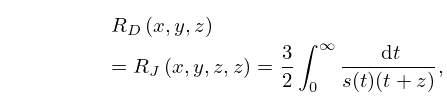
►A fourth integral that is symmetric in only two variables is defined by
►
19.16.5
…
►
19.16.15
…
►
19.16.21
…
14: 19.23 Integral Representations
…
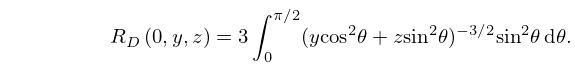
►
19.23.3
…
►In (19.23.8)–(19.23.10) one or more of the variables may be 0 if the integral converges.
…
15: 29.7 Asymptotic Expansions
…
►Müller (1966a, b) found three formal asymptotic expansions for a fundamental system of solutions of (29.2.1) (and (29.11.1)) as , one in terms of Jacobian elliptic functions and two in terms of Hermite polynomials.
…
16: 35.2 Laplace Transform
…
►where the integration variable
ranges over the space .
►Suppose there exists a constant such that for all .
…
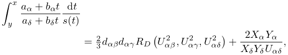
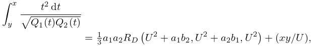
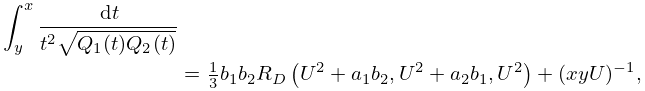
17: 19.29 Reduction of General Elliptic Integrals
…
►
19.29.7
.
…
►
19.29.10
,
…
►
19.29.20
…
►
19.29.21
…
►If both square roots in (19.29.22) are 0, then the indeterminacy in the two preceding equations can be removed by using (19.27.8) to evaluate the integral as multiplied either by or by
in the cases of (19.29.20) or (19.29.21), respectively.
…
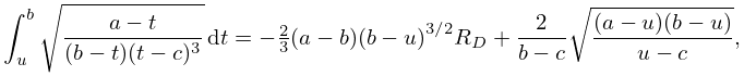
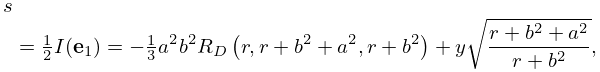
18: 19.30 Lengths of Plane Curves
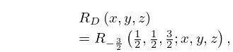
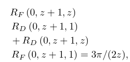
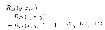
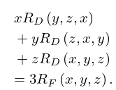
19: 19.21 Connection Formulas
…
►
19.21.1
.
…
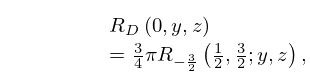
►
19.21.2
…
►
19.21.8
►
19.21.9
…
►For each value of , permutation of produces three values of , one of which lies in the same region as and two lie in the other region of the same type.
…
