functions Fℓ(η,ρ),Gℓ(η,ρ),H±ℓ(η,ρ)

(0.014 seconds)

31—40 of 236 matching pages

31: 9.18 Tables

… ►

•

Miller (1946) tabulates $\operatorname{Ai}\left(x\right)$ , $\operatorname{Ai}'\left(x\right)$ for $x=-20(.01)2;$ $\operatorname{log}_{10}\operatorname{Ai}\left(x\right)$ , $\operatorname{Ai}'\left(x\right)/\operatorname{Ai}\left(x\right)$ for $x=0(.1)25(1)75$ ; $\operatorname{Bi}\left(x\right)$ , $\operatorname{Bi}'\left(x\right)$ for $x=-10(.1)2.5$ ; $\operatorname{log}_{10}\operatorname{Bi}\left(x\right)$ , $\operatorname{Bi}'\left(x\right)/\operatorname{Bi}\left(x\right)$ for $x=0(.1)10$ ; $M\left(x\right)$ , $N\left(x\right)$ , $\theta\left(x\right)$ , $\phi\left(x\right)$ (respectively $F(x)$ , $G(x)$ , $\chi(x)$ , $\psi(x)$ ) for $x=-80(1)-30(.1)0$ . Precision is generally 8D; slightly less for some of the auxiliary functions. Extracts from these tables are included in Abramowitz and Stegun (1964, Chapter 10), together with some auxiliary functions for large arguments.

…

32: 19.4 Derivatives and Differential Equations

… ►

19.4.5

\frac{\partial F\left(\phi,k\right)}{\partial k}={\frac{E\left(\phi,k\right)-{% k^{\prime}}^{2}F\left(\phi,k\right)}{k{k^{\prime}}^{2}}-\frac{k\sin\phi\cos% \phi}{{k^{\prime}}^{2}\sqrt{1-k^{2}{\sin}^{2}\phi}}},

ⓘ

Symbols:: $\cos\NVar{z}$ : cosine function, $F\left(\NVar{\phi},\NVar{k}\right)$ : Legendre’s incomplete elliptic integral of the first kind, $E\left(\NVar{\phi},\NVar{k}\right)$ : Legendre’s incomplete elliptic integral of the second kind, $\frac{\partial\NVar{f}}{\partial\NVar{x}}$ : partial derivative of $f$ with respect to $x$ , $\,\partial\NVar{x}$ : partial differential of $x$ , $\sin\NVar{z}$ : sine function, $\phi$ : real or complex argument, $k$ : real or complex modulus and $k^{\prime}$ : complementary modulus
Permalink:: http://dlmf.nist.gov/19.4.E5
Encodings:: pMML, png, TeX
See also:: Annotations for §19.4(i), §19.4 and Ch.19

… ►

19.4.8

(k{k^{\prime}}^{2}D_{k}^{2}+(1-3k^{2})D_{k}-k)F\left(\phi,k\right)=\frac{-k% \sin\phi\cos\phi}{(1-k^{2}{\sin}^{2}\phi)^{3/2}},

ⓘ

Symbols:: $\cos\NVar{z}$ : cosine function, $F\left(\NVar{\phi},\NVar{k}\right)$ : Legendre’s incomplete elliptic integral of the first kind, $\sin\NVar{z}$ : sine function, $\phi$ : real or complex argument, $k$ : real or complex modulus, $k^{\prime}$ : complementary modulus and $D_{k}$ : differential operator
Referenced by:: §19.4(ii)
Permalink:: http://dlmf.nist.gov/19.4.E8
Encodings:: pMML, png, TeX
See also:: Annotations for §19.4(ii), §19.4 and Ch.19

…

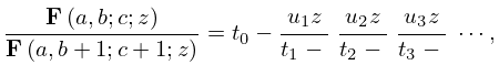
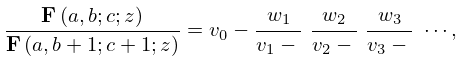
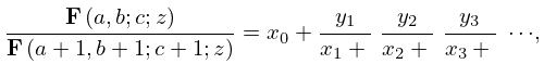
33: 15.7 Continued Fractions

… ►

15.7.1

\frac{\mathbf{F}\left(a,b;c;z\right)}{\mathbf{F}\left(a,b+1;c+1;z\right)}=t_{0% }-\cfrac{u_{1}z}{t_{1}-\cfrac{u_{2}z}{t_{2}-\cfrac{u_{3}z}{t_{3}-\cdots}}},

ⓘ

Symbols:: $\mathbf{F}\left(\NVar{a},\NVar{b};\NVar{c};\NVar{z}\right)$ or $\mathbf{F}\left({\NVar{a},\NVar{b}\atop\NVar{c}};\NVar{z}\right)$ : $={{}_{2}{\mathbf{F}}_{1}}\left(\NVar{a},\NVar{b};\NVar{c};\NVar{z}\right)$ Olver’s hypergeometric function, $z$ : complex variable, $a$ : real or complex parameter, $b$ : real or complex parameter, $c$ : real or complex parameter, $t_{n}$ : coefficient and $u_{n}$ : coefficient
Permalink:: http://dlmf.nist.gov/15.7.E1
Encodings:: pMML, png, TeX
See also:: Annotations for §15.7 and Ch.15

… ►

15.7.3

\frac{\mathbf{F}\left(a,b;c;z\right)}{\mathbf{F}\left(a,b+1;c+1;z\right)}=v_{0% }-\cfrac{w_{1}}{v_{1}-\cfrac{w_{2}}{v_{2}-\cfrac{w_{3}}{v_{3}-\cdots}}},

ⓘ

Symbols:: $\mathbf{F}\left(\NVar{a},\NVar{b};\NVar{c};\NVar{z}\right)$ or $\mathbf{F}\left({\NVar{a},\NVar{b}\atop\NVar{c}};\NVar{z}\right)$ : $={{}_{2}{\mathbf{F}}_{1}}\left(\NVar{a},\NVar{b};\NVar{c};\NVar{z}\right)$ Olver’s hypergeometric function, $z$ : complex variable, $a$ : real or complex parameter, $b$ : real or complex parameter, $c$ : real or complex parameter, $v_{n}$ : coefficient and $w_{n}$ : coefficient
Permalink:: http://dlmf.nist.gov/15.7.E3
Encodings:: pMML, png, TeX
See also:: Annotations for §15.7 and Ch.15

… ►

15.7.5

\frac{\mathbf{F}\left(a,b;c;z\right)}{\mathbf{F}\left(a+1,b+1;c+1;z\right)}={x% _{0}+\cfrac{y_{1}}{x_{1}+\cfrac{y_{2}}{x_{2}+\cfrac{y_{3}}{x_{3}+\cdots}}}},

ⓘ

Symbols:: $\mathbf{F}\left(\NVar{a},\NVar{b};\NVar{c};\NVar{z}\right)$ or $\mathbf{F}\left({\NVar{a},\NVar{b}\atop\NVar{c}};\NVar{z}\right)$ : $={{}_{2}{\mathbf{F}}_{1}}\left(\NVar{a},\NVar{b};\NVar{c};\NVar{z}\right)$ Olver’s hypergeometric function, $x$ : real variable, $y$ : real variable, $z$ : complex variable, $a$ : real or complex parameter, $b$ : real or complex parameter and $c$ : real or complex parameter
Permalink:: http://dlmf.nist.gov/15.7.E5
Encodings:: pMML, png, TeX
See also:: Annotations for §15.7 and Ch.15

…

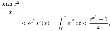
34: 7.8 Inequalities

… ►

7.8.7

\frac{\sinh x^{2}}{x}<{\mathrm{e}}^{x^{2}}F\left(x\right)=\int_{0}^{x}{\mathrm% {e}}^{t^{2}}\,\mathrm{d}t<\frac{{\mathrm{e}}^{x^{2}}-1}{x},

x>0

ⓘ

Symbols:: $F\left(\NVar{z}\right)$ : Dawson’s integral, $\,\mathrm{d}\NVar{x}$ : differential of $x$ , $\mathrm{e}$ : base of natural logarithm, $\sinh\NVar{z}$ : hyperbolic sine function, $\int$ : integral and $x$ : real variable
Referenced by:: Erratum (V1.1.5) for Additions
Permalink:: http://dlmf.nist.gov/7.8.E7
Encodings:: pMML, png, TeX
Addition (effective with 1.1.5):: A new inequality was added.
See also:: Annotations for §7.8 and Ch.7

►The function

F\left(x\right)/\sqrt{1-{\mathrm{e}}^{-2x^{2}}}

is strictly decreasing for

x>0

. …

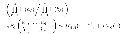
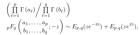
35: 16.11 Asymptotic Expansions

… ►

16.11.6

\left({\textstyle\ifrac{\prod\limits_{\ell=1}^{q+1}\Gamma\left(a_{\ell}\right)% }{\prod\limits_{\ell=1}^{q}\Gamma\left(b_{\ell}\right)}}\right){{}_{q+1}F_{q}}% \left({a_{1},\dots,a_{q+1}\atop b_{1},\dots,b_{q}};z\right)=H_{q+1,q}(-z),

|\operatorname{ph}\left(-z\right)|\leq\pi

;

ⓘ

Symbols:: $\Gamma\left(\NVar{z}\right)$ : gamma function, ${{}_{\NVar{p}}F_{\NVar{q}}}\left(\NVar{a_{1},\dots,a_{p}};\NVar{b_{1},\dots,b_% {q}};\NVar{z}\right)$ or ${{}_{\NVar{p}}F_{\NVar{q}}}\left({\NVar{a_{1},\dots,a_{p}}\atop\NVar{b_{1},% \dots,b_{q}}};\NVar{z}\right)$ : alternatively ${{}_{\NVar{p}}F_{\NVar{q}}}\left(\NVar{\mathbf{a}};\NVar{\mathbf{b}};\NVar{z}\right)$ or ${{}_{\NVar{p}}F_{\NVar{q}}}\left({\NVar{\mathbf{a}}\atop\NVar{\mathbf{b}}};% \NVar{z}\right)$
generalized hypergeometric function, $\pi$ : the ratio of the circumference of a circle to its diameter, $\operatorname{ph}$ : phase, $q$ : nonnegative integer, $z$ : complex variable, $a,a_{1},\ldots,a_{p}$ : real or complex parameters, $b,b_{1},\ldots,b_{q}$ : real or complex parameters and $H_{p,q}(z)$ : formal infinite series
Permalink:: http://dlmf.nist.gov/16.11.E6
Encodings:: pMML, png, TeX
See also:: Annotations for §16.11(ii), §16.11(ii), §16.11 and Ch.16

… ►

16.11.7

\left({\textstyle\ifrac{\prod\limits_{\ell=1}^{q}\Gamma\left(a_{\ell}\right)}{% \prod\limits_{\ell=1}^{q}\Gamma\left(b_{\ell}\right)}}\right){{}_{q}F_{q}}% \left({a_{1},\dots,a_{q}\atop b_{1},\dots,b_{q}};z\right)\sim H_{q,q}(z{% \mathrm{e}}^{\mp\pi\mathrm{i}})+E_{q,q}(z).

ⓘ

Symbols:: $\Gamma\left(\NVar{z}\right)$ : gamma function, ${{}_{\NVar{p}}F_{\NVar{q}}}\left(\NVar{a_{1},\dots,a_{p}};\NVar{b_{1},\dots,b_% {q}};\NVar{z}\right)$ or ${{}_{\NVar{p}}F_{\NVar{q}}}\left({\NVar{a_{1},\dots,a_{p}}\atop\NVar{b_{1},% \dots,b_{q}}};\NVar{z}\right)$ : alternatively ${{}_{\NVar{p}}F_{\NVar{q}}}\left(\NVar{\mathbf{a}};\NVar{\mathbf{b}};\NVar{z}\right)$ or ${{}_{\NVar{p}}F_{\NVar{q}}}\left({\NVar{\mathbf{a}}\atop\NVar{\mathbf{b}}};% \NVar{z}\right)$
generalized hypergeometric function, $\sim$ : Poincaré asymptotic expansion, $\pi$ : the ratio of the circumference of a circle to its diameter, $\mathrm{e}$ : base of natural logarithm, $\mathrm{i}$ : imaginary unit, $q$ : nonnegative integer, $z$ : complex variable, $a,a_{1},\ldots,a_{p}$ : real or complex parameters, $b,b_{1},\ldots,b_{q}$ : real or complex parameters, $E_{p,q}(z)$ : formal infinite series and $H_{p,q}(z)$ : formal infinite series
Referenced by:: §16.11(ii)
Permalink:: http://dlmf.nist.gov/16.11.E7
Encodings:: pMML, png, TeX
See also:: Annotations for §16.11(ii), §16.11(ii), §16.11 and Ch.16

… ►

16.11.8

\left({\textstyle\ifrac{\prod\limits_{\ell=1}^{q-1}\Gamma\left(a_{\ell}\right)% }{\prod\limits_{\ell=1}^{q}\Gamma\left(b_{\ell}\right)}}\right){{}_{q-1}F_{q}}% \left({a_{1},\dots,a_{q-1}\atop b_{1},\dots,b_{q}};-z\right)\sim H_{q-1,q}(z)+% E_{q-1,q}(ze^{-\pi\mathrm{i}})+E_{q-1,q}(ze^{\pi\mathrm{i}}),

ⓘ

Symbols:: $\Gamma\left(\NVar{z}\right)$ : gamma function, ${{}_{\NVar{p}}F_{\NVar{q}}}\left(\NVar{a_{1},\dots,a_{p}};\NVar{b_{1},\dots,b_% {q}};\NVar{z}\right)$ or ${{}_{\NVar{p}}F_{\NVar{q}}}\left({\NVar{a_{1},\dots,a_{p}}\atop\NVar{b_{1},% \dots,b_{q}}};\NVar{z}\right)$ : alternatively ${{}_{\NVar{p}}F_{\NVar{q}}}\left(\NVar{\mathbf{a}};\NVar{\mathbf{b}};\NVar{z}\right)$ or ${{}_{\NVar{p}}F_{\NVar{q}}}\left({\NVar{\mathbf{a}}\atop\NVar{\mathbf{b}}};% \NVar{z}\right)$
generalized hypergeometric function, $\sim$ : Poincaré asymptotic expansion, $\pi$ : the ratio of the circumference of a circle to its diameter, $\mathrm{i}$ : imaginary unit, $q$ : nonnegative integer, $z$ : complex variable, $a,a_{1},\ldots,a_{p}$ : real or complex parameters, $b,b_{1},\ldots,b_{q}$ : real or complex parameters, $E_{p,q}(z)$ : formal infinite series, $H_{p,q}(z)$ : formal infinite series and $e_{k,m}$
Permalink:: http://dlmf.nist.gov/16.11.E8
Encodings:: pMML, png, TeX
See also:: Annotations for §16.11(ii), §16.11(ii), §16.11 and Ch.16

… ►

16.11.9

\left({\textstyle\ifrac{\prod\limits_{\ell=1}^{p}\Gamma\left(a_{\ell}\right)}{% \prod\limits_{\ell=1}^{q}\Gamma\left(b_{\ell}\right)}}\right){{}_{p}F_{q}}% \left({a_{1},\dots,a_{p}\atop b_{1},\dots,b_{q}};-z\right)\sim E_{p,q}(ze^{-% \pi\mathrm{i}})+E_{p,q}(ze^{\pi\mathrm{i}}),

ⓘ

Symbols:: $\Gamma\left(\NVar{z}\right)$ : gamma function, ${{}_{\NVar{p}}F_{\NVar{q}}}\left(\NVar{a_{1},\dots,a_{p}};\NVar{b_{1},\dots,b_% {q}};\NVar{z}\right)$ or ${{}_{\NVar{p}}F_{\NVar{q}}}\left({\NVar{a_{1},\dots,a_{p}}\atop\NVar{b_{1},% \dots,b_{q}}};\NVar{z}\right)$ : alternatively ${{}_{\NVar{p}}F_{\NVar{q}}}\left(\NVar{\mathbf{a}};\NVar{\mathbf{b}};\NVar{z}\right)$ or ${{}_{\NVar{p}}F_{\NVar{q}}}\left({\NVar{\mathbf{a}}\atop\NVar{\mathbf{b}}};% \NVar{z}\right)$
generalized hypergeometric function, $\sim$ : Poincaré asymptotic expansion, $\pi$ : the ratio of the circumference of a circle to its diameter, $\mathrm{i}$ : imaginary unit, $p$ : nonnegative integer, $q$ : nonnegative integer, $z$ : complex variable, $a,a_{1},\ldots,a_{p}$ : real or complex parameters, $b,b_{1},\ldots,b_{q}$ : real or complex parameters, $E_{p,q}(z)$ : formal infinite series and $e_{k,m}$
Referenced by:: §16.11(ii)
Permalink:: http://dlmf.nist.gov/16.11.E9
Encodings:: pMML, png, TeX
See also:: Annotations for §16.11(ii), §16.11(ii), §16.11 and Ch.16

… ►

16.11.11

{{}_{p}F_{q}}\left({a_{1}+r,\dots,a_{p}+r\atop b_{1}+r,\dots,b_{q}+r};z\right)% =\sum_{n=0}^{m-1}\frac{{\left(a_{1}+r\right)_{n}}\cdots{\left(a_{p}+r\right)_{% n}}}{{\left(b_{1}+r\right)_{n}}\cdots{\left(b_{q}+r\right)_{n}}}\frac{z^{n}}{n% !}+O\left(\frac{1}{r^{(q-p)m}}\right),

ⓘ

Symbols:: $O\left(\NVar{x}\right)$ : order not exceeding, ${{}_{\NVar{p}}F_{\NVar{q}}}\left(\NVar{a_{1},\dots,a_{p}};\NVar{b_{1},\dots,b_% {q}};\NVar{z}\right)$ or ${{}_{\NVar{p}}F_{\NVar{q}}}\left({\NVar{a_{1},\dots,a_{p}}\atop\NVar{b_{1},% \dots,b_{q}}};\NVar{z}\right)$ : alternatively ${{}_{\NVar{p}}F_{\NVar{q}}}\left(\NVar{\mathbf{a}};\NVar{\mathbf{b}};\NVar{z}\right)$ or ${{}_{\NVar{p}}F_{\NVar{q}}}\left({\NVar{\mathbf{a}}\atop\NVar{\mathbf{b}}};% \NVar{z}\right)$
generalized hypergeometric function, ${\left(\NVar{a}\right)_{\NVar{n}}}$ : Pochhammer’s symbol (or shifted factorial), $!$ : factorial (as in $n!$ ), $p$ : nonnegative integer, $q$ : nonnegative integer, $z$ : complex variable, $a,a_{1},\ldots,a_{p}$ : real or complex parameters, $b,b_{1},\ldots,b_{q}$ : real or complex parameters and $r$ : large parameter
Permalink:: http://dlmf.nist.gov/16.11.E11
Encodings:: pMML, png, TeX
See also:: Annotations for §16.11(iii), §16.11 and Ch.16

…

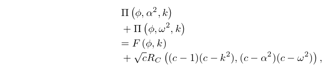
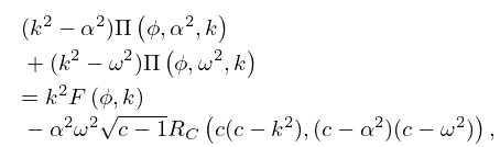
36: 19.7 Connection Formulas

… ►

19.7.8

\Pi\left(\phi,\alpha^{2},k\right)+\Pi\left(\phi,\omega^{2},k\right)=F\left(% \phi,k\right)+\sqrt{c}R_{C}\left((c-1)(c-k^{2}),(c-\alpha^{2})(c-\omega^{2})% \right),

\alpha^{2}\omega^{2}=k^{2}

ⓘ

Defines:: $\omega^{2}$ : change of variable (locally)
Symbols:: $R_{C}\left(\NVar{x},\NVar{y}\right)$ : Carlson’s combination of inverse circular and inverse hyperbolic functions, $F\left(\NVar{\phi},\NVar{k}\right)$ : Legendre’s incomplete elliptic integral of the first kind, $\Pi\left(\NVar{\phi},\NVar{\alpha}^{2},\NVar{k}\right)$ : Legendre’s incomplete elliptic integral of the third kind, $\phi$ : real or complex argument, $k$ : real or complex modulus, $\alpha^{2}$ : real or complex parameter and $c$ : change of variable
Referenced by:: §19.25(i), §19.6(i)
Permalink:: http://dlmf.nist.gov/19.7.E8
Encodings:: pMML, png, TeX
See also:: Annotations for §19.7(iii), §19.7 and Ch.19

… ►

19.7.9

(k^{2}-\alpha^{2})\Pi\left(\phi,\alpha^{2},k\right)+(k^{2}-\omega^{2})\Pi\left% (\phi,\omega^{2},k\right)=k^{2}F\left(\phi,k\right)-\alpha^{2}\omega^{2}\sqrt{% c-1}R_{C}\left(c(c-k^{2}),(c-\alpha^{2})(c-\omega^{2})\right),

(1-\alpha^{2})(1-\omega^{2})=1-k^{2}

ⓘ

Defines:: $\omega^{2}$ : change of variable (locally)
Symbols:: $R_{C}\left(\NVar{x},\NVar{y}\right)$ : Carlson’s combination of inverse circular and inverse hyperbolic functions, $F\left(\NVar{\phi},\NVar{k}\right)$ : Legendre’s incomplete elliptic integral of the first kind, $\Pi\left(\NVar{\phi},\NVar{\alpha}^{2},\NVar{k}\right)$ : Legendre’s incomplete elliptic integral of the third kind, $\phi$ : real or complex argument, $k$ : real or complex modulus, $\alpha^{2}$ : real or complex parameter and $c$ : change of variable
Permalink:: http://dlmf.nist.gov/19.7.E9
Encodings:: pMML, png, TeX
See also:: Annotations for §19.7(iii), §19.7 and Ch.19

… ►

19.7.10

(1-\alpha^{2})\Pi\left(\phi,\alpha^{2},k\right)+(1-\omega^{2})\Pi\left(\phi,% \omega^{2},k\right)=F\left(\phi,k\right)+(1-\alpha^{2}-\omega^{2})\sqrt{c-k^{2% }}\*R_{C}\left(c(c-1),(c-\alpha^{2})(c-\omega^{2})\right),

(k^{2}-\alpha^{2})(k^{2}-\omega^{2})=k^{2}(k^{2}-1)

ⓘ

Defines:: $\omega^{2}$ : change of variable (locally)
Symbols:: $R_{C}\left(\NVar{x},\NVar{y}\right)$ : Carlson’s combination of inverse circular and inverse hyperbolic functions, $F\left(\NVar{\phi},\NVar{k}\right)$ : Legendre’s incomplete elliptic integral of the first kind, $\Pi\left(\NVar{\phi},\NVar{\alpha}^{2},\NVar{k}\right)$ : Legendre’s incomplete elliptic integral of the third kind, $\phi$ : real or complex argument, $k$ : real or complex modulus, $\alpha^{2}$ : real or complex parameter and $c$ : change of variable
Permalink:: http://dlmf.nist.gov/19.7.E10
Encodings:: pMML, png, TeX
See also:: Annotations for §19.7(iii), §19.7 and Ch.19

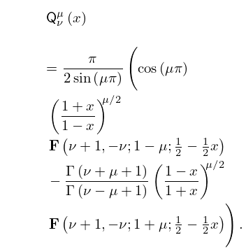
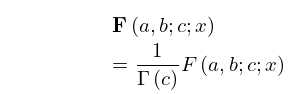
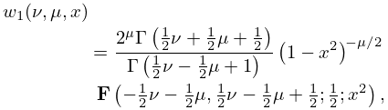
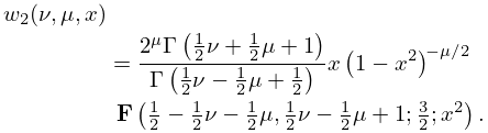
37: 14.3 Definitions and Hypergeometric Representations

… ►

14.3.2

\mathsf{Q}^{\mu}_{\nu}\left(x\right)=\frac{\pi}{2\sin\left(\mu\pi\right)}\left% (\cos\left(\mu\pi\right)\left(\frac{1+x}{1-x}\right)^{\mu/2}\mathbf{F}\left(% \nu+1,-\nu;1-\mu;\tfrac{1}{2}-\tfrac{1}{2}x\right)-\frac{\Gamma\left(\nu+\mu+1% \right)}{\Gamma\left(\nu-\mu+1\right)}\left(\frac{1-x}{1+x}\right)^{\mu/2}% \mathbf{F}\left(\nu+1,-\nu;1+\mu;\tfrac{1}{2}-\tfrac{1}{2}x\right)\right).

ⓘ

Defines:: $\mathsf{Q}^{\NVar{\mu}}_{\NVar{\nu}}\left(\NVar{x}\right)$ : Ferrers function of the second kind
Symbols:: $\Gamma\left(\NVar{z}\right)$ : gamma function, $\pi$ : the ratio of the circumference of a circle to its diameter, $\cos\NVar{z}$ : cosine function, $\mathbf{F}\left(\NVar{a},\NVar{b};\NVar{c};\NVar{z}\right)$ or $\mathbf{F}\left({\NVar{a},\NVar{b}\atop\NVar{c}};\NVar{z}\right)$ : $={{}_{2}{\mathbf{F}}_{1}}\left(\NVar{a},\NVar{b};\NVar{c};\NVar{z}\right)$ Olver’s hypergeometric function, $\sin\NVar{z}$ : sine function, $\mu$ : general order, $\nu$ : general degree and $x$ : real variable $1<x<1$
Referenced by:: §14.3(i)
Permalink:: http://dlmf.nist.gov/14.3.E2
Encodings:: pMML, png, TeX
See also:: Annotations for §14.3(i), §14.3(i), §14.3 and Ch.14

… ►

14.3.3

\mathbf{F}\left(a,b;c;x\right)=\frac{1}{\Gamma\left(c\right)}F\left(a,b;c;x\right)

ⓘ

Symbols:: $\Gamma\left(\NVar{z}\right)$ : gamma function, $F\left(\NVar{a},\NVar{b};\NVar{c};\NVar{z}\right)$ or $F\left({\NVar{a},\NVar{b}\atop\NVar{c}};\NVar{z}\right)$ : $={{}_{2}F_{1}}\left(\NVar{a},\NVar{b};\NVar{c};\NVar{z}\right)$ Gauss’ hypergeometric function, $\mathbf{F}\left(\NVar{a},\NVar{b};\NVar{c};\NVar{z}\right)$ or $\mathbf{F}\left({\NVar{a},\NVar{b}\atop\NVar{c}};\NVar{z}\right)$ : $={{}_{2}{\mathbf{F}}_{1}}\left(\NVar{a},\NVar{b};\NVar{c};\NVar{z}\right)$ Olver’s hypergeometric function and $x$ : real variable $1<x<1$
Permalink:: http://dlmf.nist.gov/14.3.E3
Encodings:: pMML, png, TeX
See also:: Annotations for §14.3(i), §14.3(i), §14.3 and Ch.14

… ►

14.3.13

w_{1}(\nu,\mu,x)=\frac{2^{\mu}\Gamma\left(\frac{1}{2}\nu+\frac{1}{2}\mu+\frac{% 1}{2}\right)}{\Gamma\left(\frac{1}{2}\nu-\frac{1}{2}\mu+1\right)}\left(1-x^{2}% \right)^{-\mu/2}\mathbf{F}\left(-\tfrac{1}{2}\nu-\tfrac{1}{2}\mu,\tfrac{1}{2}% \nu-\tfrac{1}{2}\mu+\tfrac{1}{2};\tfrac{1}{2};x^{2}\right),

ⓘ

Symbols:: $\Gamma\left(\NVar{z}\right)$ : gamma function, $\mathbf{F}\left(\NVar{a},\NVar{b};\NVar{c};\NVar{z}\right)$ or $\mathbf{F}\left({\NVar{a},\NVar{b}\atop\NVar{c}};\NVar{z}\right)$ : $={{}_{2}{\mathbf{F}}_{1}}\left(\NVar{a},\NVar{b};\NVar{c};\NVar{z}\right)$ Olver’s hypergeometric function, $x$ : real variable, $\mu$ : general order, $\nu$ : general degree and $w_{2}$ : function $w_{1}$ ,
Referenced by:: §10.59
Permalink:: http://dlmf.nist.gov/14.3.E13
Encodings:: pMML, png, TeX
See also:: Annotations for §14.3(iii), §14.3 and Ch.14

►

14.3.14

w_{2}(\nu,\mu,x)=\frac{2^{\mu}\Gamma\left(\frac{1}{2}\nu+\frac{1}{2}\mu+1% \right)}{\Gamma\left(\frac{1}{2}\nu-\frac{1}{2}\mu+\frac{1}{2}\right)}x\left(1% -x^{2}\right)^{-\mu/2}\mathbf{F}\left(\tfrac{1}{2}-\tfrac{1}{2}\nu-\tfrac{1}{2% }\mu,\tfrac{1}{2}\nu-\tfrac{1}{2}\mu+1;\tfrac{3}{2};x^{2}\right).

ⓘ

Symbols:: $\Gamma\left(\NVar{z}\right)$ : gamma function, $\mathbf{F}\left(\NVar{a},\NVar{b};\NVar{c};\NVar{z}\right)$ or $\mathbf{F}\left({\NVar{a},\NVar{b}\atop\NVar{c}};\NVar{z}\right)$ : $={{}_{2}{\mathbf{F}}_{1}}\left(\NVar{a},\NVar{b};\NVar{c};\NVar{z}\right)$ Olver’s hypergeometric function, $x$ : real variable, $\mu$ : general order, $\nu$ : general degree and $w_{2}$ : function $w_{1}$ ,
Referenced by:: §10.59, §14.3(i), §14.5(i)
Permalink:: http://dlmf.nist.gov/14.3.E14
Encodings:: pMML, png, TeX
See also:: Annotations for §14.3(iii), §14.3 and Ch.14

… ►

14.3.19

\boldsymbol{Q}^{\mu}_{\nu}\left(x\right)=\frac{2^{\nu}\Gamma\left(\nu+1\right)% (x+1)^{\mu/2}}{(x-1)^{(\mu/2)+\nu+1}}\mathbf{F}\left(\nu+1,\nu+\mu+1;2\nu+2;% \frac{2}{1-x}\right),

ⓘ

Symbols:: $\Gamma\left(\NVar{z}\right)$ : gamma function, $\boldsymbol{Q}^{\NVar{\mu}}_{\NVar{\nu}}\left(\NVar{z}\right)$ : Olver’s associated Legendre function, $\mathbf{F}\left(\NVar{a},\NVar{b};\NVar{c};\NVar{z}\right)$ or $\mathbf{F}\left({\NVar{a},\NVar{b}\atop\NVar{c}};\NVar{z}\right)$ : $={{}_{2}{\mathbf{F}}_{1}}\left(\NVar{a},\NVar{b};\NVar{c};\NVar{z}\right)$ Olver’s hypergeometric function, $\mu$ : general order, $\nu$ : general degree and $x$ : real variable $x>1$
Permalink:: http://dlmf.nist.gov/14.3.E19
Encodings:: pMML, png, TeX
See also:: Annotations for §14.3(iii), §14.3 and Ch.14

…

38: 19.37 Tables

… ►

Functions $F\left(\phi,k\right)$ and $E\left(\phi,k\right)$

… ►

Functions $R_{F}\left(x^{2},1,y^{2}\right)$ and $R_{G}\left(x^{2},1,y^{2}\right)$

… ►

Function $R_{F}\left(a^{2},b^{2},c^{2}\right)$ with $abc=1$

…

39: 7.24 Approximations

… ►

•

Cody et al. (1970) gives minimax rational approximations to Dawson’s integral $F\left(x\right)$ (maximum relative precision 20S–22S).

… ►

•

Luke (1969b, pp. 323–324) covers $\frac{1}{2}\sqrt{\pi}\operatorname{erf}x$ and $e^{x^{2}}F\left(x\right)$ for $-3\leq x\leq 3$ (the Chebyshev coefficients are given to 20D); $\sqrt{\pi}xe^{x^{2}}\operatorname{erfc}x$ and $2xF\left(x\right)$ for $x\geq 3$ (the Chebyshev coefficients are given to 20D and 15D, respectively). Coefficients for the Fresnel integrals are given on pp. 328–330 (20D).

… ►

•

Luke (1969b, vol. 2, pp. 422–435) gives main diagonal Padé approximations for $F\left(z\right)$ , $\operatorname{erf}z$ , $\operatorname{erfc}z$ , $C\left(z\right)$ , and $S\left(z\right)$ ; approximate errors are given for a selection of $z$ -values.

40: 1.6 Vectors and Vector-Valued Functions

… ►The divergence of a differentiable vector-valued function

\mathbf{F}=F_{1}\mathbf{i}+F_{2}\mathbf{j}+F_{3}\mathbf{k}

is … ►The curl of

\mathbf{F}

is … ►The line integral of a vector-valued function

\mathbf{F}=F_{1}\mathbf{i}+F_{2}\mathbf{j}+F_{3}\mathbf{k}

along

\mathbf{c}

is given by … ►For a vector-valued function

\mathbf{F}

, … ►when

\mathbf{F}

is a continuously differentiable vector-valued function. …