fractional transformations
(0.002 seconds)
21—30 of 32 matching pages
21: Bibliography W
…
►
Analytic Theory of Continued Fractions.
D. Van Nostrand Company, Inc., New York.
…
►
The cubic transformation of the hypergeometric function.
Quart. J. Pure and Applied Math. 41, pp. 70–79.
…
►
Some transformations of generalized hypergeometric series.
Proc. London Math. Soc. (2) 26 (2), pp. 257–272.
…
►
The Airy transform.
Amer. Math. Monthly 86 (4), pp. 271–277.
►
The Laplace Transform.
Princeton Mathematical Series, v. 6, Princeton University Press, Princeton, NJ.
…
22: Bibliography G
…
►
Contiguous relations and summation and transformation formulae for basic hypergeometric series.
J. Difference Equ. Appl. 19 (12), pp. 2029–2042.
…
►
A continued fraction algorithm for the computation of higher transcendental functions in the complex plane.
Math. Comp. 21 (97), pp. 18–29.
…
►
Formulas of the Dirichlet-Mehler Type.
In Fractional Calculus and its Applications, B. Ross (Ed.),
Lecture Notes in Math., Vol. 457, pp. 207–215.
…
►
Problem 72-21, Laplace transforms of Airy functions.
SIAM Rev. 15 (4), pp. 796–798.
…
►
Fourier transforms related to a root system of rank 1.
Transform. Groups 12 (1), pp. 77–116.
…
23: 15.6 Integral Representations
…
►
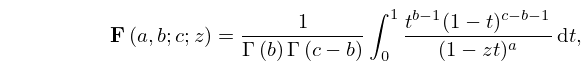
15.6.1
; .
►
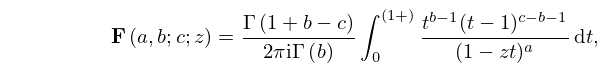
15.6.2
; , .
►
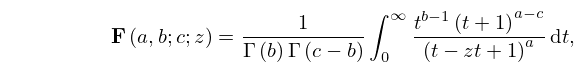
15.6.2_5
; .
…
►
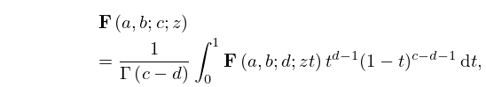
15.6.8
; .
…
►Note that (15.6.8) can be rewritten as a fractional integral.
…
24: Bibliography O
…
►
Tables of Lebedev, Mehler and Generalized Mehler Transforms.
Mathematical Note
Technical Report 246, Boeing Scientific Research Lab, Seattle.
►
Tables of Fourier Transforms and Fourier Transforms of Distributions.
Springer-Verlag, Berlin.
…
►
Tables of Bessel Transforms.
Springer-Verlag, Berlin-New York.
…
►
Tables of Mellin Transforms.
Springer-Verlag, Berlin-New York.
…
►
Second-order differential equations with fractional transition points.
Trans. Amer. Math. Soc. 226, pp. 227–241.
…
25: 1.15 Summability Methods
…
►where is the Fourier transform of (§1.14(i)).
…
►
§1.15(vi) Fractional Integrals
►For and , the Riemann-Liouville fractional integral of order is defined by … ►§1.15(vii) Fractional Derivatives
… ►Note that . …26: 3.11 Approximation Techniques
…
►
Laplace Transform Inversion
►Numerical inversion of the Laplace transform (§1.14(iii)) … ►Example. The Discrete Fourier Transform
… ►is called a discrete Fourier transform pair. ►The Fast Fourier Transform
…27: 10.74 Methods of Computation
…
►
§10.74(v) Continued Fractions
… ►Hankel Transform
… ►Spherical Bessel Transform
►The spherical Bessel transform is the Hankel transform (10.22.76) in the case when is half an odd positive integer. … ►Kontorovich–Lebedev Transform
…28: 20.11 Generalizations and Analogs
…
►If both are positive, then allows inversion of its arguments as a modular transformation (compare (23.15.3) and (23.15.4)):
…
►In the case identities for theta functions become identities in the complex variable , with , that involve rational functions, power series, and continued fractions; see Adiga et al. (1985), McKean and Moll (1999, pp. 156–158), and Andrews et al. (1988, §10.7).
…
29: 13.4 Integral Representations
…
►The fractional powers are continuous and assume their principal values at .
…At this point the fractional powers are determined by and .
…
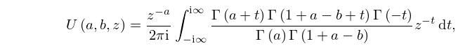
►
13.4.16
,
…
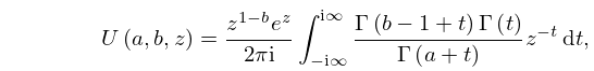
►
13.4.17
,
…
►
13.4.18
,
…
30: Bibliography R
…
►
A code to calculate (high order) Bessel functions based on the continued fractions method.
Comput. Phys. Comm. 76 (3), pp. 381–388.
…
►
Partial fractions expansions and identities for products of Bessel functions.
J. Math. Phys. 46 (4), pp. 043509–1–043509–18.
…
►
Finite-sum rules for Macdonald’s functions and Hankel’s symbols.
Integral Transform. Spec. Funct. 10 (2), pp. 115–124.
…
