fractional integrals

(0.004 seconds)

21—30 of 64 matching pages

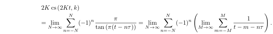
21: 22.12 Expansions in Other Trigonometric Series and Doubly-Infinite Partial Fractions: Eisenstein Series

… ►

22.12.13

2K\operatorname{cs}\left(2Kt,k\right)=\lim_{N\to\infty}\sum_{n=-N}^{N}(-1)^{n}% \frac{\pi}{\tan\left(\pi(t-n\tau)\right)}=\lim_{N\to\infty}\sum_{n=-N}^{N}(-1)% ^{n}\left(\lim_{M\to\infty}\sum_{m=-M}^{M}\frac{1}{t-m-n\tau}\right).

ⓘ

Symbols:: $\operatorname{cs}\left(\NVar{z},\NVar{k}\right)$ : Jacobian elliptic function, $\pi$ : the ratio of the circumference of a circle to its diameter, $K\left(\NVar{k}\right)$ : Legendre’s complete elliptic integral of the first kind, $\tan\NVar{z}$ : tangent function, $k$ : modulus and $\tau$ : ratio
Referenced by:: §22.12
Permalink:: http://dlmf.nist.gov/22.12.E13
Encodings:: pMML, png, TeX
See also:: Annotations for §22.12 and Ch.22

22: 5.12 Beta Function

… ►In this section all fractional powers have their principal values, except where noted otherwise. … ►

Euler’s Beta Integral

… ►In (5.12.8) the fractional powers have their principal values when

w>0

and

z>0

, and are continued via continuity. … ►In (5.12.11) and (5.12.12) the fractional powers are continuous on the integration paths and take their principal values at the beginning. … ►

Pochhammer’s Integral

…

23: 5.9 Integral Representations

§5.9 Integral Representations

… ►(The fractional powers have their principal values.) ►

Hankel’s Loop Integral

… ► … ► …

24: 14.32 Methods of Computation

… ►

•

Quadrature (§3.5) of the integral representations given in §§14.12, 14.19(iii), 14.20(iv), and 14.25; see Segura and Gil (1999) and Gil et al. (2000).

►

•

Evaluation (§3.10) of the continued fractions given in §14.14. See Gil and Segura (2000).

…

25: 18.40 Methods of Computation

… ►The problem of moments is simply stated and the early work of Stieltjes, Markov, and Chebyshev on this problem was the origin of the understanding of the importance of both continued fractions and OP’s in many areas of analysis. … ►The question is then: how is this possible given only

F_{N}(z)

, rather than

F(z)

itself?

F_{N}(z)

often converges to smooth results for

z

off the real axis for

\Im{z}

at a distance greater than the pole spacing of the

x_{n}

, this may then be followed by approximate numerical analytic continuation via fitting to lower order continued fractions (either Padé, see §3.11(iv), or pointwise continued fraction approximants, see Schlessinger (1968, Appendix)), to

F_{N}(z)

and evaluating these on the real axis in regions of higher pole density that those of the approximating function. … ►Equation (18.40.7) provides step-histogram approximations to

\int_{a}^{x}\,\mathrm{d}\mu(x)

, as shown in Figure 18.40.1 for

N=12

and

120

, shown here for the repulsive Coulomb–Pollaczek OP’s of Figure 18.39.2, with the parameters as listed therein. … ►The bottom and top of the steps at the

x_{i}

are lower and upper bounds to

\int_{a}^{x_{i}}\,\mathrm{d}\mu(x)

as made explicit via the Chebyshev inequalities discussed by Shohat and Tamarkin (1970, pp. 42–43). … ►In what follows this is accomplished in two ways: i) via the Lagrange interpolation of §3.3(i) ; and ii) by constructing a pointwise continued fraction, or PWCF, as follows: …

26: 13.4 Integral Representations

§13.4 Integral Representations

… ►

§13.4(ii) Contour Integrals

… ►The fractional powers are continuous and assume their principal values at

t=\alpha

. …At this point the fractional powers are determined by

\operatorname{ph}{t}=\pi

and

\operatorname{ph}\left(1+t\right)=0

. … ►

27: 6.18 Methods of Computation

§6.18 Methods of Computation

… ►Quadrature of the integral representations is another effective method. … ►Lastly, the continued fraction (6.9.1) can be used if

|z|

is bounded away from the origin. … ►

§6.18(ii) Auxiliary Functions

… ►

§6.18(iii) Zeros

…

28: 19.14 Reduction of General Elliptic Integrals

§19.14 Reduction of General Elliptic Integrals

… ►Legendre (1825–1832) showed that every elliptic integral can be expressed in terms of the three integrals in (19.1.2) supplemented by algebraic, logarithmic, and trigonometric functions. …The last reference gives a clear summary of the various steps involving linear fractional transformations, partial-fraction decomposition, and recurrence relations. It then improves the classical method by first applying Hermite reduction to (19.2.3) to arrive at integrands without multiple poles and uses implicit full partial-fraction decomposition and implicit root finding to minimize computing with algebraic extensions. …

29: 3.10 Continued Fractions

§3.10 Continued Fractions

… ►

Stieltjes Fractions

… ►is called a Stieltjes fraction ( $S$ -fraction). … ►

Jacobi Fractions

… ►The continued fraction …

30: Bibliography G

… ►

I. Gargantini and P. Henrici (1967) A continued fraction algorithm for the computation of higher transcendental functions in the complex plane. Math. Comp. 21 (97), pp. 18–29.

ⓘ

External Links:: FullText, MathReview (D. C. Gilles), ZentralBlatt
Referenced by:: §10.74(v), §3.10(ii).
Encodings:: BibTeX

… ►

G. Gasper (1975) Formulas of the Dirichlet-Mehler Type. In Fractional Calculus and its Applications, B. Ross (Ed.), Lecture Notes in Math., Vol. 457, pp. 207–215.

ⓘ