differences

SearchAdvancedHelp

(0.000 seconds)

21—30 of 176 matching pages

21: 27.22 Software

… ►

Mathematica. PrimeQ combines strong pseudoprime tests for the bases 2 and 3 and a Lucas pseudoprime test. No known composite numbers pass these three tests, and Bleichenbacher (1996) has shown that this combination of tests proves primality for integers below ${10}^{16}$. Provable PrimeQ uses the Atkin–Goldwasser–Kilian–Morain Elliptic Curve Method to prove primality. FactorInteger tries Brent–Pollard rho, Pollard $p-1$, and then cfrac after trial division. See §27.19. ecm is available also, and the Multiple Polynomial Quadratic sieve is expected in a future release.

For additional Mathematica routines for factorization and primality testing, including several different pseudoprime tests, see Bressoud and Wagon (2000).

…

22: 11.13 Methods of Computation

… ►

§11.13(v) Difference Equations

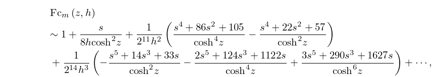
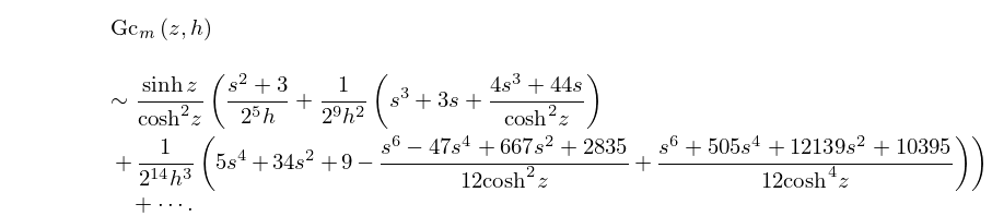
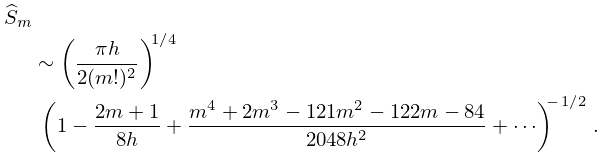
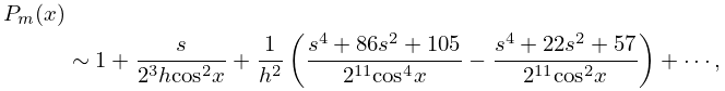
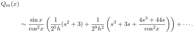
►Sequences of values of ${𝐇}_{\nu }\left(z\right)$ and ${𝐋}_{\nu }\left(z\right)$, with $z$ fixed, can be computed by application of the inhomogeneous difference equations (11.4.23) and (11.4.25). …

23: 28.26 Asymptotic Approximations for Large $q$

… ►

28.26.1 $${\mathrm{Mc}}_m^{(3)}(z,h)=\frac{{\mathrm{e}}^{\mathrm{i}\varphi }}{{(\pi h\cosh z)}^{1/2}}\left({\mathrm{Fc}}_m(z,h)-\mathrm{i}{\mathrm{Gc}}_m(z,h)\right),$$

ⓘ

Symbols:

$\pi$: the ratio of the circumference of a circle to its diameter, $\mathrm{e}$: base of natural logarithm, $\cosh z$: hyperbolic cosine function, $\mathrm{i}$: imaginary unit, ${\mathrm{Mc}}_n^{(j)}(z,h)$: radial Mathieu function, $m$: integer, $h$: parameter, $z$: complex variable and $\varphi$

A&S Ref:

20.9.7 (in slightly different notation)

Permalink:

http://dlmf.nist.gov/28.26.E1

Encodings:

pMML, png, TeX

See also:

Annotations for §28.26(i), §28.26 and Ch.28

►

28.26.2 $$\mathrm{i}{\mathrm{Ms}}_{m+1}^{(3)}(z,h)=\frac{{\mathrm{e}}^{\mathrm{i}\varphi }}{{(\pi h\cosh z)}^{1/2}}\left({\mathrm{Fs}}_m(z,h)-\mathrm{i}{\mathrm{Gs}}_m(z,h)\right),$$

ⓘ

Symbols:

$\pi$: the ratio of the circumference of a circle to its diameter, $\mathrm{e}$: base of natural logarithm, $\cosh z$: hyperbolic cosine function, $\mathrm{i}$: imaginary unit, ${\mathrm{Ms}}_n^{(j)}(z,h)$: radial Mathieu function, $m$: integer, $h$: parameter, $z$: complex variable and $\varphi$

A&S Ref:

20.9.7 (in slightly different notation)

Permalink:

http://dlmf.nist.gov/28.26.E2

Encodings:

pMML, png, TeX

See also:

Annotations for §28.26(i), §28.26 and Ch.28

… ►

28.26.3 $$\varphi =2h\sinh z-\left(m+\frac{1}{2}\right)\arctan \left(\sinh z\right).$$

ⓘ

Symbols:

$\sinh z$: hyperbolic sine function, $\arctan z$: arctangent function, $m$: integer, $h$: parameter, $z$: complex variable and $\varphi$

A&S Ref:

20.9.8 (in slightly different notation)

Permalink:

http://dlmf.nist.gov/28.26.E3

Encodings:

pMML, png, TeX

See also:

Annotations for §28.26(i), §28.26 and Ch.28

… ►

28.26.4 $${\mathrm{Fc}}_m(z,h)\sim 1+\frac{s}{8h{\cosh }^{2}z}+\frac{1}{2^{11}{h}^2}\left(\frac{s^4+86s^2+105}{{\cosh }^{4}z}-\frac{s^4+22s^2+57}{{\cosh }^{2}z}\right)+\frac{1}{2^{14}{h}^3}\left(-\frac{s^5+14s^3+33s}{{\cosh }^{2}z}-\frac{2s^5+124s^3+1122s}{{\cosh }^{4}z}+\frac{3s^5+290s^3+1627s}{{\cosh }^{6}z}\right)+\mathrm{\cdots },$$

ⓘ

Symbols:

$\sim$: Poincaré asymptotic expansion, $\cosh z$: hyperbolic cosine function, $m$: integer, $h$: parameter and $z$: complex variable

A&S Ref:

20.9.9 (in slightly different notation)

Referenced by:

§28.26(i)

Permalink:

http://dlmf.nist.gov/28.26.E4

Encodings:

pMML, png, TeX

See also:

Annotations for §28.26(i), §28.26 and Ch.28

►

28.26.5 $${\mathrm{Gc}}_m(z,h)\sim \frac{\sinh z}{{\cosh }^{2}z}\left(\frac{s^2+3}{2^{5}h}+\frac{1}{2^9{h}^2}\left(s^3+3s+\frac{4s^3+44s}{{\cosh }^{2}z}\right)+\frac{1}{2^{14}{h}^3}\left(5s^4+34s^2+9-\frac{s^6-47s^4+667s^2+2835}{12{\cosh }^{2}z}+\frac{s^6+505s^4+12139s^2+10395}{12{\cosh }^{4}z}\right)\right)+\mathrm{\cdots }.$$

ⓘ

Symbols:

$\sim$: Poincaré asymptotic expansion, $\cosh z$: hyperbolic cosine function, $\sinh z$: hyperbolic sine function, $m$: integer, $h$: parameter and $z$: complex variable

A&S Ref:

20.9.10 (in slightly different notation)

Referenced by:

§28.26(i)

Permalink:

http://dlmf.nist.gov/28.26.E5

Encodings:

pMML, png, TeX

See also:

Annotations for §28.26(i), §28.26 and Ch.28

…

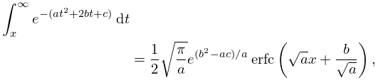
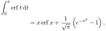
24: 7.7 Integral Representations

… ►

7.7.1 $$\mathrm{erfc}z=\frac{2}{\pi }{\mathrm{e}}^{-z^2}{\int }_0^{\mathrm{\infty }}\frac{{\mathrm{e}}^{-z^2{t}^2}}{t^2+1}dt,$$ $|\mathrm{ph}z|\le \frac{1}{4}\pi$,

ⓘ

Symbols:

$\pi$: the ratio of the circumference of a circle to its diameter, $\mathrm{erfc}z$: complementary error function, $dx$: differential of $x$ , $\mathrm{e}$: base of natural logarithm, $\int$: integral, $\mathrm{ph}$: phase and $z$: complex variable

A&S Ref:

7.4.11 (in different form)

Referenced by:

§7.11, §7.7(i)

Permalink:

http://dlmf.nist.gov/7.7.E1

Encodings:

pMML, png, TeX

See also:

Annotations for §7.7(i), §7.7 and Ch.7

►

7.7.2 $$w\left(z\right)=\frac{1}{\pi \mathrm{i}}{\int }_{-\mathrm{\infty }}^{\mathrm{\infty }}\frac{{\mathrm{e}}^{-t^2}dt}{t-z}=\frac{2z}{\pi \mathrm{i}}{\int }_0^{\mathrm{\infty }}\frac{{\mathrm{e}}^{-t^2}dt}{t^2-z^2},$$ $\mathrm{\Im }z>0$.

ⓘ

Symbols:

$\pi$: the ratio of the circumference of a circle to its diameter, $dx$: differential of $x$ , $w\left(z\right)$: Faddeeva (or Faddeyeva) function, $\mathrm{e}$: base of natural logarithm, $\mathrm{\Im }$: imaginary part, $\mathrm{i}$: imaginary unit, $\int$: integral and $z$: complex variable

A&S Ref:

7.1.4 (in different form)

Referenced by:

§7.19(i), §7.22(i), §7.7(i)

Permalink:

http://dlmf.nist.gov/7.7.E2

Encodings:

pMML, png, TeX

See also:

Annotations for §7.7(i), §7.7 and Ch.7

►

7.7.3 $${\int }_0^{\mathrm{\infty }}{\mathrm{e}}^{-a{t}^2+2\mathrm{i}zt}dt=\frac{1}{2}\sqrt{\frac{\pi }{a}}{\mathrm{e}}^{-z^2/a}+\frac{\mathrm{i}}{\sqrt{a}}F\left(\frac{z}{\sqrt{a}}\right),$$ $\mathrm{\Re }a>0$.

ⓘ

Symbols:

$F\left(z\right)$: Dawson’s integral, $\pi$: the ratio of the circumference of a circle to its diameter, $dx$: differential of $x$ , $\mathrm{e}$: base of natural logarithm, $\mathrm{i}$: imaginary unit, $\int$: integral, $\mathrm{\Re }$: real part and $z$: complex variable

A&S Ref:

7.4.6 7.4.7 (in different notation)

Referenced by:

§7.14(i), §7.7(i)

Permalink:

http://dlmf.nist.gov/7.7.E3

Encodings:

pMML, png, TeX

See also:

Annotations for §7.7(i), §7.7 and Ch.7

… ►

7.7.6 $${\int }_x^{\mathrm{\infty }}{\mathrm{e}}^{-(a{t}^2+2bt+c)}dt=\frac{1}{2}\sqrt{\frac{\pi }{a}}{\mathrm{e}}^{(b^2-ac)/a}\mathrm{erfc}\left(\sqrt{a}x+\frac{b}{\sqrt{a}}\right),$$ $\mathrm{\Re }a>0$.

ⓘ

Symbols:

$\pi$: the ratio of the circumference of a circle to its diameter, $\mathrm{erfc}z$: complementary error function, $dx$: differential of $x$ , $\mathrm{e}$: base of natural logarithm, $\int$: integral, $\mathrm{\Re }$: real part and $x$: real variable

A&S Ref:

7.4.32 (in different form)

Referenced by:

§7.14(i), §7.7(i)

Permalink:

http://dlmf.nist.gov/7.7.E6

Encodings:

pMML, png, TeX

See also:

Annotations for §7.7(i), §7.7 and Ch.7

… ►

7.7.9 $${\int }_0^x\mathrm{erf}tdt=x\mathrm{erf}x+\frac{1}{\sqrt{\pi }}\left({\mathrm{e}}^{-x^2}-1\right).$$

ⓘ

Symbols:

$\pi$: the ratio of the circumference of a circle to its diameter, $dx$: differential of $x$ , $\mathrm{erf}z$: error function, $\mathrm{e}$: base of natural logarithm, $\int$: integral and $x$: real variable

A&S Ref:

7.4.35 (in different form)

Referenced by:

§7.7(i)

Permalink:

http://dlmf.nist.gov/7.7.E9

Encodings:

pMML, png, TeX

See also:

Annotations for §7.7(i), §7.7 and Ch.7

…

25: Mathematical Introduction

… ►Two other ways in which this Handbook differs from AMS 55, and other handbooks, are as follows. … ►These include, for example, multivalued functions of complex variables, for which new definitions of branch points and principal values are supplied (§§1.10(vi), 4.2(i)); the Dirac delta (or delta function), which is introduced in a more readily comprehensible way for mathematicians (§1.17); numerically satisfactory solutions of differential and difference equations (§§2.7(iv), 2.9(i)); and numerical analysis for complex variables (Chapter 3). … ► ►►►►

$ℂ$	complex plane (excluding infinity).
…
$\mathrm{\Delta }$ (or ${\mathrm{\Delta }}_x$)	forward difference operator: $\mathrm{\Delta }f(x)=f(x+1)-f(x)$.
$\nabla$ (or ${\nabla }_x$)	backward difference operator: $\nabla f(x)=f(x)-f(x-1)$. (See also del operator in the Notations section.)
…

…

26: 18.19 Hahn Class: Definitions

… ►The Askey scheme extends the three families of classical OP’s (Jacobi, Laguerre and Hermite) with eight further families of OP’s for which the role of the differentiation operator $\frac{d}{dx}$ in the case of the classical OP’s is played by a suitable difference operator. … ►

Hahn class (or linear lattice class). These are OP’s $p_n(x)$ where the role of $\frac{d}{dx}$ is played by ${\mathrm{\Delta }}_x$ or ${\nabla }_x$ or ${\delta }_x$ (see §18.1(i) for the definition of these operators). The Hahn class consists of four discrete and two continuous families.

►

Wilson class (or quadratic lattice class). These are OP’s $p_n(x)=p_n(\lambda (y))$ ($p_n(x)$ of degree $n$ in $x$, $\lambda (y)$ quadratic in $y$) where the role of the differentiation operator is played by $\frac{{\mathrm{\Delta }}_y}{{\mathrm{\Delta }}_y(\lambda (y))}$ or $\frac{{\nabla }_y}{{\nabla }_y(\lambda (y))}$ or $\frac{{\delta }_y}{{\delta }_y(\lambda (y))}$. The Wilson class consists of two discrete and two continuous families.

…

27: 28.8 Asymptotic Expansions for Large $q$

… ►

28.8.6 $${\widehat{C}}_m\sim {\left(\frac{\pi h}{2{(m!)}^2}\right)}^{1/4}{\left(1+\frac{2m+1}{8h}+\frac{m^4+2m^3+263m^2+262m+108}{2048h^2}+\mathrm{\cdots }\right)}^{-1/2},$$

ⓘ

Defines:

${\widehat{C}}_m$: coefficient (locally)

Symbols:

$\sim$: Poincaré asymptotic expansion, $\pi$: the ratio of the circumference of a circle to its diameter, $!$: factorial (as in $n!$), $m$: integer and $h$: parameter

A&S Ref:

20.9.19 (in slightly different form)

Permalink:

http://dlmf.nist.gov/28.8.E6

Encodings:

pMML, png, TeX

See also:

Annotations for §28.8(ii), §28.8 and Ch.28

►

28.8.7 $${\widehat{S}}_m\sim {\left(\frac{\pi h}{2{(m!)}^2}\right)}^{1/4}{\left(1-\frac{2m+1}{8h}+\frac{m^4+2m^3-121m^2-122m-84}{2048h^2}+\mathrm{\cdots }\right)}^{-1/2}.$$

ⓘ

Defines:

${\widehat{S}}_m$: coefficient (locally)

Symbols:

$\sim$: Poincaré asymptotic expansion, $\pi$: the ratio of the circumference of a circle to its diameter, $!$: factorial (as in $n!$), $m$: integer and $h$: parameter

A&S Ref:

20.9.20 (in slightly different form)

Referenced by:

§28.8(ii), Erratum (V1.1.10) for Sections 28.6(i), 28.6(ii), 28.8(i), 28.8(ii)

Permalink:

http://dlmf.nist.gov/28.8.E7

Encodings:

pMML, png, TeX

See also:

Annotations for §28.8(ii), §28.8 and Ch.28

… ►

28.8.9 $$W_m^{\pm }(x)=\frac{{\mathrm{e}}^{\pm 2h\sin x}}{{(\cos x)}^{m+1}}\{\begin{array}{cc}{\left(\cos \left(\frac{1}{2}x+\frac{1}{4}\pi \right)\right)}^{2m+1},\hfill & \\ {\left(\sin \left(\frac{1}{2}x+\frac{1}{4}\pi \right)\right)}^{2m+1},\hfill & \end{array}$$

ⓘ

Defines:

$W_m^{\pm }$: function (locally)

Symbols:

$\pi$: the ratio of the circumference of a circle to its diameter, $\cos z$: cosine function, $\mathrm{e}$: base of natural logarithm, $\sin z$: sine function, $m$: integer, $h$: parameter and $x$: real variable

A&S Ref:

20.9.13 (in slightly different form)

Permalink:

http://dlmf.nist.gov/28.8.E9

Encodings:

pMML, png, TeX

See also:

Annotations for §28.8(iii), §28.8 and Ch.28

… ►

28.8.11 $$P_m(x)\sim 1+\frac{s}{2^{3}h{\cos }^{2}x}+\frac{1}{h^2}\left(\frac{s^4+86s^2+105}{2^{11}{\cos }^{4}x}-\frac{s^4+22s^2+57}{2^{11}{\cos }^{2}x}\right)+\mathrm{\cdots },$$

ⓘ

Defines:

$P_m(x)$ (locally)

Symbols:

$\sim$: Poincaré asymptotic expansion, $\cos z$: cosine function, $m$: integer, $h$: parameter and $x$: real variable

A&S Ref:

20.9.14 (in different form)

Permalink:

http://dlmf.nist.gov/28.8.E11

Encodings:

pMML, png, TeX

See also:

Annotations for §28.8(iii), §28.8 and Ch.28

►

28.8.12 $$Q_m(x)\sim \frac{\sin x}{{\cos }^{2}x}\left(\frac{1}{2^{5}h}(s^2+3)+\frac{1}{2^9{h}^2}\left(s^3+3s+\frac{4s^3+44s}{{\cos }^{2}x}\right)\right)+\mathrm{\cdots }.$$

ⓘ

Defines:

$Q_m(x)$ (locally)

Symbols:

$\sim$: Poincaré asymptotic expansion, $\cos z$: cosine function, $\sin z$: sine function, $m$: integer, $h$: parameter and $x$: real variable

A&S Ref:

20.9.14 (in different form)

Permalink:

http://dlmf.nist.gov/28.8.E12

Encodings:

pMML, png, TeX

See also:

Annotations for §28.8(iii), §28.8 and Ch.28

…

28: Guide to Searching the DLMF

… ►To recognize the math symbols and structures, and to accommodate equivalence between various notations and various forms of expression, the search system maps the math part of your queries into a different form. … ►DLMF search is generally case-insensitive except when it is important to be case-sensitive, as when two different special functions have the same standard names but one name has a lower-case initial and the other is has an upper-case initial, such as si and Si, gamma and Gamma. … ►DLMF search recognizes just the essential font differences, that is, the font style differences deemed important for the DLMF contents: …

29: 20.2 Definitions and Periodic Properties

… ►

20.2.5 $$z_{m,n}=(m+n\tau )\pi ,$$ $m,n\in \mathbb{Z}$,

ⓘ

Symbols:

$\pi$: the ratio of the circumference of a circle to its diameter, $\in$: element of, $\mathbb{Z}$: set of all integers, $m$: integer, $n$: integer, $z$: complex and $\tau$: lattice parameter

A&S Ref:

16.33.1 (in different notation)

Referenced by:

§20.6

Permalink:

http://dlmf.nist.gov/20.2.E5

Encodings:

pMML, png, TeX

See also:

Annotations for §20.2(ii), §20.2 and Ch.20

… ►

20.2.6 $${\theta }_1\left(z+(m+n\tau )\pi \right|\tau )={(-1)}^{m+n}{q}^{-n^2}{\mathrm{e}}^{-2\mathrm{i}nz}{\theta }_1\left(z\right|\tau ),$$

ⓘ

Symbols:

${\theta }_j\left(z\right|\tau )$: theta function, $\pi$: the ratio of the circumference of a circle to its diameter, $\mathrm{e}$: base of natural logarithm, $\mathrm{i}$: imaginary unit, $m$: integer, $n$: integer, $z$: complex, $\tau$: lattice parameter and $q$: nome

A&S Ref:

16.33.2 (in different notation)

Referenced by:

§23.6(i)

Permalink:

http://dlmf.nist.gov/20.2.E6

Encodings:

pMML, png, TeX

See also:

Annotations for §20.2(ii), §20.2 and Ch.20

►

20.2.7 $${\theta }_2\left(z+(m+n\tau )\pi \right|\tau )={(-1)}^m{q}^{-n^2}{\mathrm{e}}^{-2\mathrm{i}nz}{\theta }_2\left(z\right|\tau ),$$

ⓘ

Symbols:

${\theta }_j\left(z\right|\tau )$: theta function, $\pi$: the ratio of the circumference of a circle to its diameter, $\mathrm{e}$: base of natural logarithm, $\mathrm{i}$: imaginary unit, $m$: integer, $n$: integer, $z$: complex, $\tau$: lattice parameter and $q$: nome

A&S Ref:

16.33.3 (in different notation)

Permalink:

http://dlmf.nist.gov/20.2.E7

Encodings:

pMML, png, TeX

See also:

Annotations for §20.2(ii), §20.2 and Ch.20

►

20.2.8 $${\theta }_3\left(z+(m+n\tau )\pi \right|\tau )=q^{-n^2}{\mathrm{e}}^{-2\mathrm{i}nz}{\theta }_3\left(z\right|\tau ),$$

ⓘ

Symbols:

${\theta }_j\left(z\right|\tau )$: theta function, $\pi$: the ratio of the circumference of a circle to its diameter, $\mathrm{e}$: base of natural logarithm, $\mathrm{i}$: imaginary unit, $m$: integer, $n$: integer, $z$: complex, $\tau$: lattice parameter and $q$: nome

A&S Ref:

16.33.4 (in different notation)

Permalink:

http://dlmf.nist.gov/20.2.E8

Encodings:

pMML, png, TeX

See also:

Annotations for §20.2(ii), §20.2 and Ch.20

… ►

20.2.10 $$M\equiv M(z|\tau )={\mathrm{e}}^{\mathrm{i}z+(\mathrm{i}\pi \tau /4)},$$

ⓘ

Defines:

$M$ (locally)

Symbols:

$\pi$: the ratio of the circumference of a circle to its diameter, $\equiv$: equals by definition, $\mathrm{e}$: base of natural logarithm, $\mathrm{i}$: imaginary unit, $z$: complex and $\tau$: lattice parameter

A&S Ref:

16.33.1 (in different notation)

Permalink:

http://dlmf.nist.gov/20.2.E10

Encodings:

pMML, png, TeX

See also:

Annotations for §20.2(iii), §20.2 and Ch.20

…

30: 28.10 Integral Equations

… ►

28.10.1 $$\frac{2}{\pi }{\int }_0^{\pi /2}\cos \left(2h\cos z\cos t\right){\mathrm{ce}}_{2n}(t,h^2)dt=\frac{A_0^{2n}(h^2)}{{\mathrm{ce}}_{2n}(\frac{1}{2}\pi ,h^2)}{\mathrm{ce}}_{2n}(z,h^2),$$

ⓘ

Symbols:

${\mathrm{ce}}_n(z,q)$: Mathieu function, $\pi$: the ratio of the circumference of a circle to its diameter, $\cos z$: cosine function, $dx$: differential of $x$ , $\int$: integral, $h$: parameter, $n$: integer, $z$: complex variable and $A_m(q)$: Fourier coefficient

A&S Ref:

20.7.20 (in different form)

Permalink:

http://dlmf.nist.gov/28.10.E1

Encodings:

pMML, png, TeX

See also:

Annotations for §28.10(i), §28.10 and Ch.28

►

28.10.2 $$\frac{2}{\pi }{\int }_0^{\pi /2}\cosh \left(2h\sin z\sin t\right){\mathrm{ce}}_{2n}(t,h^2)dt=\frac{A_0^{2n}(h^2)}{{\mathrm{ce}}_{2n}(0,h^2)}{\mathrm{ce}}_{2n}(z,h^2),$$

ⓘ

Symbols:

${\mathrm{ce}}_n(z,q)$: Mathieu function, $\pi$: the ratio of the circumference of a circle to its diameter, $dx$: differential of $x$ , $\cosh z$: hyperbolic cosine function, $\int$: integral, $\sin z$: sine function, $h$: parameter, $n$: integer, $z$: complex variable and $A_m(q)$: Fourier coefficient

A&S Ref:

20.7.21 (in different form)

Permalink:

http://dlmf.nist.gov/28.10.E2

Encodings:

pMML, png, TeX

See also:

Annotations for §28.10(i), §28.10 and Ch.28

►

28.10.3 $$\frac{2}{\pi }{\int }_0^{\pi /2}\sin \left(2h\cos z\cos t\right){\mathrm{ce}}_{2n+1}(t,h^2)dt=-\frac{h{A}_1^{2n+1}(h^2)}{{\mathrm{ce}}_{2n+1}^{\prime }(\frac{1}{2}\pi ,h^2)}{\mathrm{ce}}_{2n+1}(z,h^2),$$

ⓘ

Symbols:

${\mathrm{ce}}_n(z,q)$: Mathieu function, $\pi$: the ratio of the circumference of a circle to its diameter, $\cos z$: cosine function, $dx$: differential of $x$ , $\int$: integral, $\sin z$: sine function, $h$: parameter, $n$: integer, $z$: complex variable and $A_m(q)$: Fourier coefficient

A&S Ref:

20.7.20 (in different form)

Permalink:

http://dlmf.nist.gov/28.10.E3

Encodings:

pMML, png, TeX

See also:

Annotations for §28.10(i), §28.10 and Ch.28

►

28.10.4 $$\frac{2}{\pi }{\int }_0^{\pi /2}\cos z\cos t\cosh \left(2h\sin z\sin t\right){\mathrm{ce}}_{2n+1}(t,h^2)dt=\frac{A_1^{2n+1}(h^2)}{2{\mathrm{ce}}_{2n+1}(0,h^2)}{\mathrm{ce}}_{2n+1}(z,h^2),$$

ⓘ

Symbols:

${\mathrm{ce}}_n(z,q)$: Mathieu function, $\pi$: the ratio of the circumference of a circle to its diameter, $\cos z$: cosine function, $dx$: differential of $x$ , $\cosh z$: hyperbolic cosine function, $\int$: integral, $\sin z$: sine function, $h$: parameter, $n$: integer, $z$: complex variable and $A_m(q)$: Fourier coefficient

A&S Ref:

20.7.21 (in different form)

Permalink:

http://dlmf.nist.gov/28.10.E4

Encodings:

pMML, png, TeX

See also:

Annotations for §28.10(i), §28.10 and Ch.28

►

28.10.5 $$\frac{2}{\pi }{\int }_0^{\pi /2}\sinh \left(2h\sin z\sin t\right){\mathrm{se}}_{2n+1}(t,h^2)dt=\frac{h{B}_1^{2n+1}(h^2)}{{\mathrm{se}}_{2n+1}^{\prime }(0,h^2)}{\mathrm{se}}_{2n+1}(z,h^2),$$

ⓘ

Symbols:

${\mathrm{se}}_n(z,q)$: Mathieu function, $\pi$: the ratio of the circumference of a circle to its diameter, $dx$: differential of $x$ , $\sinh z$: hyperbolic sine function, $\int$: integral, $\sin z$: sine function, $h$: parameter, $n$: integer, $z$: complex variable and $B_m(q)$: Fourier coefficient

A&S Ref:

20.7.23 (in different form)

Permalink:

http://dlmf.nist.gov/28.10.E5

Encodings:

pMML, png, TeX

See also:

Annotations for §28.10(i), §28.10 and Ch.28

…