cosine transform
(0.002 seconds)
11—20 of 56 matching pages
11: Guide to Searching the DLMF
…
►
Table 1: Query Examples
►
►
►
…
| Query | Matching records contain |
|---|---|
"Fourier transform" and series |
both the phrase “Fourier transform” and the word “series”. |
| … | |
Fourier (transform or series) |
at least one of “Fourier transform” or “Fourier series”. |
1/(2pi) and "Fourier transform" |
both and the phrase “Fourier transform”. |
sin^2 +cos^2 |
the expression . |
| … | |
DeMoivre and cos (n theta) |
both the word “DeMoivre” and the expression . |
| … | |
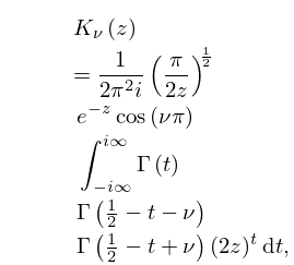
12: 10.32 Integral Representations
…
►
10.32.14
.
…
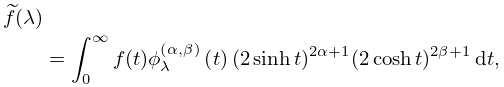
13: 15.9 Relations to Other Functions
…
►The Jacobi transform is defined as
►
15.9.12
►with inverse
…
…
►Any hypergeometric function for which a quadratic transformation exists can be expressed in terms of associated Legendre functions or Ferrers functions.
…
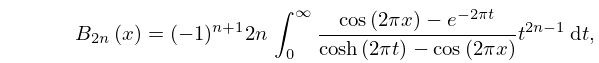
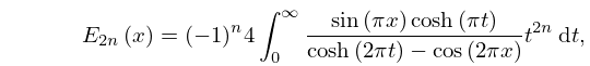
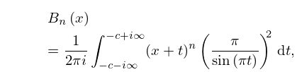
14: 24.7 Integral Representations
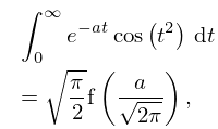
15: 7.7 Integral Representations
…
►
7.7.15
,
…
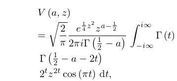
16: 12.5 Integral Representations
…
►
12.5.9
,
,
…
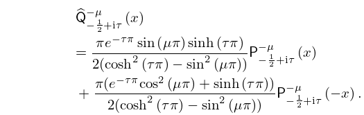
17: 14.20 Conical (or Mehler) Functions
…
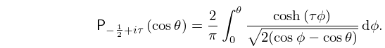
►
14.20.3
…
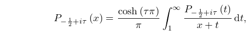
►
14.20.9
…
►From (14.20.9) or (14.20.10) it is evident that is positive for real .
►
§14.20(vi) Generalized Mehler–Fock Transformation
… ►
14.20.13
…
18: Bibliography F
…
►
Un théorème de Paley-Wiener pour la transformation de Fourier sur un espace riemannien symétrique de rang un.
J. Funct. Anal. 49 (2), pp. 230–268.
…
►
Calculation of elliptic integrals of the third kind by means of Gauss’ transformation.
Math. Comp. 19 (89), pp. 97–104.
…
►
Numerical calculation of singular integrals related to Hankel transform.
Comput. Math. Appl. 21 (2-3), pp. 87–94.
…
►
On a unified approach to transformations and elementary solutions of Painlevé equations.
J. Math. Phys. 23 (11), pp. 2033–2042.
…
►
On the asymptotic expansion of Mellin transforms.
SIAM J. Math. Anal. 18 (1), pp. 273–282.
…
