closed point set

SearchAdvancedHelp

(0.005 seconds)

11—20 of 56 matching pages

11: 36.15 Methods of Computation

… ►Close to the origin $𝐱=\mathrm{𝟎}$ of parameter space, the series in §36.8 can be used. … ►Far from the bifurcation set, the leading-order asymptotic formulas of §36.11 reproduce accurately the form of the function, including the geometry of the zeros described in §36.7. Close to the bifurcation set but far from $𝐱=\mathrm{𝟎}$, the uniform asymptotic approximations of §36.12 can be used. … ►Direct numerical evaluation can be carried out along a contour that runs along the segment of the real $t$-axis containing all real critical points of $\mathrm{\Phi }$ and is deformed outside this range so as to reach infinity along the asymptotic valleys of $\exp \left(\mathrm{i}\mathrm{\Phi }\right)$. … ►This can be carried out by direct numerical evaluation of canonical integrals along a finite segment of the real axis including all real critical points of $\mathrm{\Phi }$, with contributions from the contour outside this range approximated by the first terms of an asymptotic series associated with the endpoints. …

12: 1.5 Calculus of Two or More Variables

… ►A function is continuous on a point set $D$ if it is continuous at all points of $D$. … … ►Suppose that $a,b,c$ are finite, $d$ is finite or $+\mathrm{\infty }$, and $f(x,y)$, $\partial f/\partial x$ are continuous on the partly-closed rectangle or infinite strip $[a,b]\times [c,d)$. … ►let $({\xi }_j,{\eta }_k)$ denote any point in the rectangle $[x_j,x_{j+1}]\times [y_k,y_{k+1}]$, $j=0,\mathrm{\dots },n-1$, $k=0,\mathrm{\dots },m-1$. … ►Again the mapping is one-to-one except perhaps for a set of points of volume zero. …

13: 21.1 Special Notation

… ► ►►►►►►

$g,h$	positive integers.
…
$𝜶,𝜷$	$g$-dimensional vectors, with all elements in $[0,1)$, unless stated otherwise.
…
$S^g$	set of $g$-dimensional vectors with elements in $S$.
…
$S_1/S_2$	set of all elements of $S_1$, modulo elements of $S_2$. Thus two elements of $S_1/S_2$ are equivalent if they are both in $S_1$ and their difference is in $S_2$. (For an example see §20.12(ii).)
$a\circ b$	intersection index of $a$ and $b$, two cycles lying on a closed surface. $a\circ b=0$ if $a$ and $b$ do not intersect. Otherwise $a\circ b$ gets an additive contribution from every intersection point. This contribution is $1$ if the basis of the tangent vectors of the $a$ and $b$ cycles (§21.7(i)) at the point of intersection is positively oriented; otherwise it is $-1$.
…

… ►The function $\mathrm{\Theta }(\mathit{\varphi }|𝐁)=\theta \left(\mathit{\varphi }/(2\pi \mathrm{i})\right|𝐁/(2\pi \mathrm{i}))$ is also commonly used; see, for example, Belokolos et al. (1994, §2.5), Dubrovin (1981), and Fay (1973, Chapter 1).

14: 1.18 Linear Second Order Differential Operators and Eigenfunction Expansions

… ►Let $X=[a,b]$ or $[a,b)$ or $(a,b]$ or $(a,b)$ be a (possibly infinite, or semi-infinite) interval in $ℝ$. … ►Often circumstances allow rather stronger statements, such as uniform convergence, or pointwise convergence at points where $f(x)$ is continuous, with convergence to $(f(x_0-)+f(x_0+))/2$ if $x_0$ is an isolated point of discontinuity. … ►Let $T$ be a self-adjoint extension of differential operator $ℒ$ of the form (1.18.28) and assume $T$ has a complete set of $L^2$ eigenfunctions, ${\left\{{\varphi }_{{\lambda }_n}(x)\right\}}_{n=0}^{\mathrm{\infty }}$ , $x\in X=[a,b]$ this latter being an appropriate sub-set of $ℝ$, or, in some cases $X=ℝ$ itself, with real eigenvalues ${\lambda }_n$. … ►More generally, continuous spectra may occur in sets of disjoint finite intervals $[{\lambda }_a,{\lambda }_b]\in (0,\mathrm{\infty })$, often called bands, when $q(x)$ is periodic, see Ashcroft and Mermin (1976, Ch 8) and Kittel (1996, Ch 7). … ►We assume a continuous spectrum $\lambda \in {𝝈}_c=[0,\mathrm{\infty })$, and a finite or countably infinite point spectrum ${𝝈}_p$ with elements ${\lambda }_n$. …

15: 18.2 General Orthogonal Polynomials

… ►

Orthogonality on Countable Sets

►Let $X$ be a finite set of distinct points on $ℝ$, or a countable infinite set of distinct points on $ℝ$, and $w_x$, $x\in X$, be a set of positive constants. …when $X$ is a finite set of $N+1$ distinct points. … ►In further generalizations of the class $𝒮$ discrete mass points $x_k$ outside $[-1,1]$ are allowed. … ►If $d\mu \in 𝐌(a,b)$ then the interval $[b-a,b+a]$ is included in the support of $d\mu$, and outside $[b-a,b+a]$ the measure $d\mu$ only has discrete mass points $x_k$ such that $b\pm a$ are the only possible limit points of the sequence $\{x_k\}$, see Máté et al. (1991, Theorem 10). …

16: 36.7 Zeros

… ►The zeros in Table 36.7.1 are points in the $𝐱=(x,y)$ plane, where $\mathrm{ph}{\mathrm{\Psi }}_2\left(𝐱\right)$ is undetermined. …Close to the $y$-axis the approximate location of these zeros is given by … ►Deep inside the bifurcation set, that is, inside the three-cusped astroid (36.4.10) and close to the part of the $z$-axis that is far from the origin, the zero contours form an array of rings close to the planes …The rings are almost circular (radii close to $(\Delta x)/9$ and varying by less than 1%), and almost flat (deviating from the planes $z_n$ by at most $(\Delta z)/36$). …Outside the bifurcation set (36.4.10), each rib is flanked by a series of zero lines in the form of curly “antelope horns” related to the “outside” zeros (36.7.2) of the cusp canonical integral. …

17: 7.20 Mathematical Applications

… ►For applications of the complementary error function in uniform asymptotic approximations of integrals—saddle point coalescing with a pole or saddle point coalescing with an endpoint—see Wong (1989, Chapter 7), Olver (1997b, Chapter 9), and van der Waerden (1951). … ►Let the set $\{x(t),y(t),t\}$ be defined by $x(t)=C\left(t\right)$, $y(t)=S\left(t\right)$, $t\ge 0$. Then the set $\{x(t),y(t)\}$ is called Cornu’s spiral: it is the projection of the corkscrew on the $\{x,y\}$-plane. …Let $P(t)=P(x(t),y(t))$ be any point on the projected spiral. …Furthermore, because $dy/dx=\tan \left(\frac{1}{2}\pi t^2\right)$, the angle between the $x$-axis and the tangent to the spiral at $P(t)$ is given by $\frac{1}{2}\pi t^2$. …

18: 4.2 Definitions

… ►where the path does not intersect $(-\mathrm{\infty },0]$; see Figure 4.2.1. $\ln z$ is a single-valued analytic function on $ℂ\setminus (-\mathrm{\infty },0]$ and real-valued when $z$ ranges over the positive real numbers. … ►In the DLMF we allow a further extension by regarding the cut as representing two sets of points, one set corresponding to the “upper side” and denoted by $z=x+\mathrm{i}0$, the other set corresponding to the “lower side” and denoted by $z=x-\mathrm{i}0$. … ►In contrast to (4.2.5) the closed definition is symmetric. … ►This is an analytic function of $z$ on $ℂ\setminus (-\mathrm{\infty },0]$, and is two-valued and discontinuous on the cut shown in Figure 4.2.1, unless $a\in \mathbb{Z}$. …

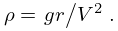
19: 36.13 Kelvin’s Ship-Wave Pattern

… ►

36.13.2 $$\rho =gr/V^2.$$

ⓘ

Symbols:

$V$: speed and $g$: gravity

Permalink:

http://dlmf.nist.gov/36.13.E2

Encodings:

pMML, png, TeX

See also:

Annotations for §36.13 and Ch.36

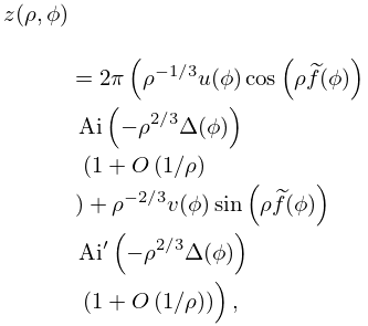
… ►When $\rho >1$, that is, everywhere except close to the ship, the integrand oscillates rapidly. There are two stationary points, given by … ►The disturbance $z(\rho ,\varphi )$ can be approximated by the method of uniform asymptotic approximation for the case of two coalescing stationary points (36.12.11), using the fact that ${\theta }_{\pm }(\varphi )$ are real for and complex for $|\varphi |>{\varphi }_c$. … ►

36.13.8 $$z(\rho ,\varphi )=2\pi \left({\rho }^{-1/3}u(\varphi )\cos \left(\rho \tilde{f}(\varphi )\right)\mathrm{Ai}\left(-{\rho }^{2/3}\mathrm{\Delta }(\varphi )\right)(1+O\left(1/\rho \right))+{\rho }^{-2/3}v(\varphi )\sin \left(\rho \tilde{f}(\varphi )\right){\mathrm{Ai}}^{\prime }\left(-{\rho }^{2/3}\mathrm{\Delta }(\varphi )\right)(1+O\left(1/\rho \right))\right),$$ $\rho \to \mathrm{\infty }$.

ⓘ

Symbols:

$\mathrm{Ai}\left(z\right)$: Airy function, $O\left(x\right)$: order not exceeding, $\pi$: the ratio of the circumference of a circle to its diameter, $\cos z$: cosine function, $\sin z$: sine function, $z(\varphi ,\rho )$: wave height approximant, $u(\varphi )$: function and $v(\varphi )$: function

Referenced by:

Figure 36.13.1, Figure 36.13.1

Permalink:

http://dlmf.nist.gov/36.13.E8

Encodings:

pMML, png, TeX

See also:

Annotations for §36.13 and Ch.36

…

20: 25.12 Polylogarithms

… ►In the complex plane ${\mathrm{Li}}_2\left(z\right)$ has a branch point at $z=1$. The principal branch has a cut along the interval $[1,\mathrm{\infty })$ and agrees with (25.12.1) when $|z|\le 1$; see also §4.2(i). … ►

25.12.3 $${\mathrm{Li}}_2\left(z\right)+{\mathrm{Li}}_2\left(\frac{z}{z-1}\right)=-\frac{1}{2}{(\ln \left(1-z\right))}^2,$$ $z\in ℂ\setminus [1,\mathrm{\infty })$.

ⓘ

Symbols:

$[a,b)$: half-closed interval, $ℂ$: complex plane, ${\mathrm{Li}}_2\left(z\right)$: dilogarithm, $\in$: element of, $\ln z$: principal branch of logarithm function, $\setminus$: set subtraction, $x$: real variable and $z$: complex variable

Keywords:

connection formula

Source:

Maximon (2003, (3.4), p. 2808)

A&S Ref:

27.7.5 (is a modified form with $z=1-x$)

Permalink:

http://dlmf.nist.gov/25.12.E3

Encodings:

pMML, png, TeX

See also:

Annotations for §25.12(i), §25.12 and Ch.25

►

25.12.4 $${\mathrm{Li}}_2\left(z\right)+{\mathrm{Li}}_2\left(\frac{1}{z}\right)=-\frac{1}{6}{\pi }^2-\frac{1}{2}{(\ln \left(-z\right))}^2,$$ $z\in ℂ\setminus [0,\mathrm{\infty })$.

ⓘ

Symbols:

$\pi$: the ratio of the circumference of a circle to its diameter, $[a,b)$: half-closed interval, $ℂ$: complex plane, ${\mathrm{Li}}_2\left(z\right)$: dilogarithm, $\in$: element of, $\ln z$: principal branch of logarithm function, $\setminus$: set subtraction and $z$: complex variable

Keywords:

connection formula

Source:

Maximon (2003, (3.2), p. 2808)

Referenced by:

§25.12(ii)

Permalink:

http://dlmf.nist.gov/25.12.E4

Encodings:

pMML, png, TeX

See also:

Annotations for §25.12(i), §25.12 and Ch.25

… ►Sometimes the factor $1/\mathrm{\Gamma }\left(s+1\right)$ is omitted. …